Logistic Regression: Predicting Outcomes with Data

SUPERCHARGE YOUR ONLINE VISIBILITY! CONTACT US AND LET’S ACHIEVE EXCELLENCE TOGETHER!

This project demonstrates how logistic regression can be used to predict outcomes in various real-life scenarios. By building a logistic regression model, we can use raw data to predict whether or not a specific event will occur. This technique is widely applicable across healthcare, finance, marketing, and e-commerce industries.

For example, logistic regression can help answer questions like:

• Will a customer default on a loan?
• Will a patient be diagnosed with a disease?
• Will a user click on an advertisement?
• Will a customer churn from a service?

This project illustrates how to apply logistic regression to analyze data, train a predictive model, and make informed decisions based on the results.

---

What is Logistic Regression?

• Logistic regression is a statistical method used to predict the probability of an event occurring. Specifically, it is a binary classification algorithm, which helps predict one of two possible outcomes, such as yes/no, true/false, or clicked/not clicked. It works by analyzing the relationship between one or more independent variables (features) and a dependent variable (outcome). Logistic regression doesn’t predict exact numbers; instead, it predicts the likelihood that a certain event will happen.

How Logistic Regression Works?

• Logistic regression uses a mathematical function called the logistic function (or sigmoid function) to convert predicted values into probabilities. The output is always between 0 and 1, which can be interpreted as a probability.

For example:

• If the probability is 0.8, there is an 80% chance that the event will happen (e.g., a customer will default on a loan).
• If the probability is 0.2, there is a 20% chance that the event will happen.

We set a threshold (commonly 0.5) to classify the results. We predict the event will occur if the probability is above the threshold (e.g., “yes”). If it’s below the threshold, we predict the event will not occur (e.g., “no”).

---

Real-Life Use Cases of Logistic Regression

Logistic regression has a wide range of use cases across different industries. Here are some real-life applications:

• Healthcare: Predicting Heart Disease In healthcare, logistic regression can predict whether a patient is at risk of developing a disease based on their medical history and test results. For example, logistic regression can predict the probability of a patient developing heart disease by analyzing factors like age, cholesterol levels, and blood pressure. This helps doctors make preventive decisions.
• Finance: Loan Default Prediction Financial institutions use logistic regression to assess the likelihood of a customer defaulting on a loan. By analyzing data like a customer’s income, credit score, and loan amount, the model can predict the probability of default, helping banks decide whether or not to approve the loan.
• Marketing: Ad Click Prediction Logistic regression is widely used in marketing to predict click-through rates (CTR). It helps advertisers understand the likelihood of a user clicking on an online advertisement based on user demographics, time spent on the page, and device type. This allows marketers to optimize their ad campaigns and target the right audience.
• E-commerce: Customer Churn Prediction E-commerce platforms use logistic regression to predict whether a customer will churn (stop using the service). By analyzing customer behavior, such as purchase history, time spent on the platform, and number of interactions, logistic regression can forecast the probability of a customer leaving the platform. Companies can then implement strategies to retain high-risk customers.

---

Critical Elements of Logistic Regression

Here are some important concepts related to logistic regression:

• Features (Independent Variables): The inputs or factors affect the outcome. For example, in predicting heart disease, features could include age, gender, cholesterol levels, etc.
• Target Variable (Dependent Variable): We are trying to predict this outcome, such as whether the patient has heart disease (1 or 0).
• Sigmoid Function: This is the core function used in logistic regression to convert the output into a probability between 0 and 1.
• Threshold: A decision boundary, usually set at 0.5, determines whether the prediction is classified as a “yes” or “no.”

---

Steps in Building a Logistic Regression Model

Below is a step-by-step outline of how we would build and apply logistic regression to a project:

• Step 1: Data Collection We start by gathering data that contains relevant features and the target variable. For example, in a heart disease prediction project, we would collect patient data, including** age, blood pressure, cholesterol levels, and whether they were diagnosed with heart disease.**
• Step 2: Data Preprocessing Preprocessing the data involves handling missing values, encoding categorical variables (e.g., converting “male/female” into 0/1), and normalizing or scaling numerical values to ensure the model performs efficiently.
• Step 3: Train-Test Split We split the data into two sets: training data (used to train the model) and testing data (used to evaluate the model). Typically, 80% of the data is used for training and 20% for testing.
• Step 4: Model Training The logistic regression model is trained on the training dataset to learn the relationships between the features and the target variable.
• Step 5: Making Predictions Once the model is trained, we use it to make predictions on the test dataset. The model outputs probabilities that can be classified as “yes” or “no” based on the threshold.
• Step 6: Model Evaluation We evaluate the model’s performance using metrics like accuracy, precision, recall, and the confusion matrix to understand how well the model predicts the outcome.

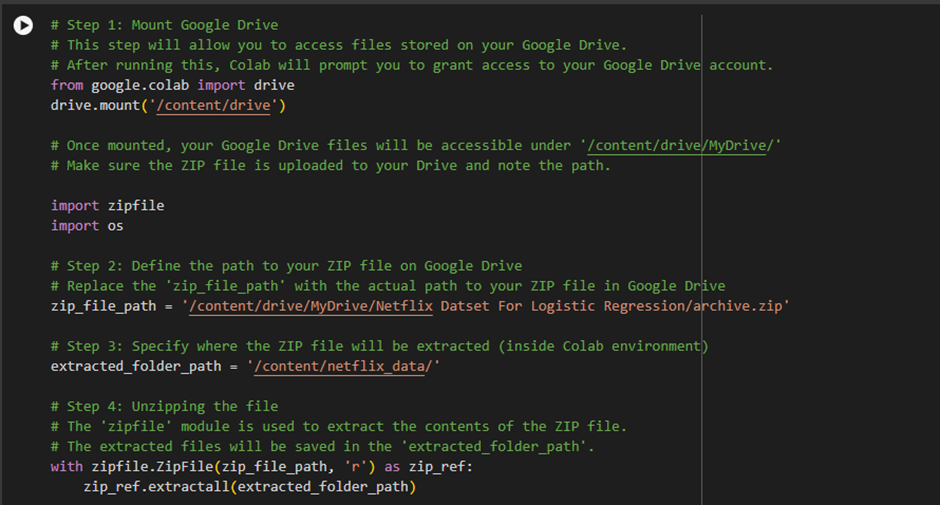
Accessing External Files:

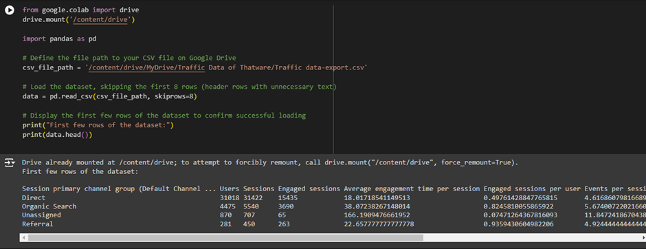
• Colab is a cloud-based environment, meaning it doesn’t automatically have access to files stored on your local machine or your Google Drive. If you have data files (e.g., CSV, ZIP) saved in your Google Drive that you want to use in Colab, you need to “mount” or connect your Google Drive to Colab so that it can access those files.

Using Data from Drive:

• If you have a dataset, a ZIP file, or any other file stored in your Google Drive, mounting it allows you to access those files as if they were part of Colab’s local file system. This makes working with large datasets you’ve already uploaded to your Drive is easy.

Saving Results Back to Drive:

• Not only can you read files from Google Drive, but you can also save output files or results back into your Google Drive. This saves model outputs, processed data, or other results you may need later.

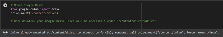
How It Works:

·         drive.mount(‘/content/drive‘): This command mounts (connects) your Google Drive to your Colab environment. Once executed, Colab will prompt you to authorize the connection by signing in to your Google account and allowing access.

·         Authorization: You’ll need to grant permission for Colab to access your Google Drive. After that, the contents of your Google Drive will be available in the Colab environment.

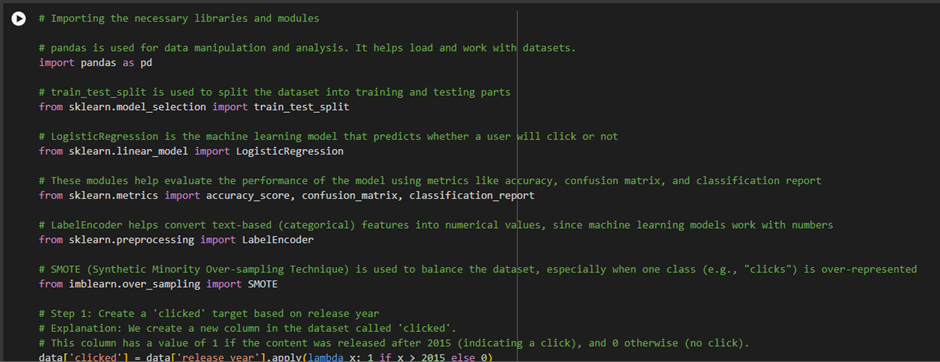
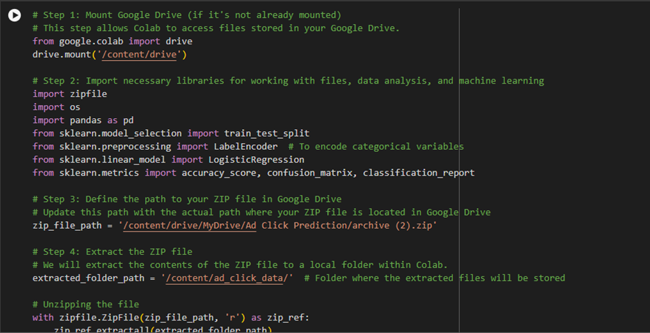
1. Import necessary libraries:

import zipfile

import os

• zipfile: This module works with ZIP files. It allows you to read, write, and extract ZIP archives.
• os: This module is used to interact with the file system. It helps navigate directories, list files, and perform other file-related operations.

2. Define the path to your ZIP file on Google Drive:

zip_file_path = ‘/content/drive/MyDrive/Ad Click Prediction/archive (2).zip’

Purpose: You’re specifying the location of the ZIP file in Google Drive.

• The zip_file_path points to the ZIP file you want to extract. This path must be the correct path where the ZIP file is located in Google Drive.
• /content/drive/MyDrive/ is the path to your Google Drive folder once mounted in Colab.
• Ad Click Prediction/archive (2).zip refers to the specific folder and ZIP file within Google Drive.

3. Specify the folder where the extracted files will be saved

extracted_folder_path = ‘/content/netflix_data/’

• Purpose: Here, you define a local folder in your Colab environment where the ZIP file’s contents will be extracted.
• /content/netflix_data/ is a directory within Colab where you want to save the extracted files.
• Colab operates in a cloud environment, so this path refers to a local folder in the Colab environment (not Google Drive).

4. Unzipping the file

with zipfile.ZipFile(zip_file_path, ‘r’) as zip_ref:

• Purpose: This step extracts the contents of the ZIP file.

How It Works:

• zipfile.ZipFile(zip_file_path, ‘r’): Opens the ZIP file in read mode (‘r’). The zip_file_path points to the file you want to extract.
• zip_ref.extractall(extracted_folder_path): Extract all the ZIP file’s contents into the specified folder (extracted_folder_path).
• The extractall() method takes the extracted contents and saves them into the folder path you defined earlier (in this case, /content/netflix_data/).

5. Listing the extracted files

extracted_files = os.listdir(extracted_folder_path)

print(“Extracted files:”, extracted_files)

8 Purpose: This step lists and prints the extracted files to ensure the ZIP file was unpacked correctly.

How It Works:

• os.listdir(extracted_folder_path): This function lists all the files in the folder /content/netflix_data/ (where the ZIP was extracted).
• print(extracted_files): Prints the names of the files to the console so you can verify that the extraction process was successful and see which files were extracted.

1. Import the pandas library

import pandas as pd

Purpose: This line imports the pandas library, a powerful Python library for data manipulation and analysis.

• pandas provide data structures like DataFrames, which make it easy to load, manipulate, and analyze tabular data (e.g., from CSV files).

2. Specify the path to the extracted CSV file

csv_file_path = ‘/content/netflix_data/netflix_titles.csv‘

Purpose: This line defines the path to the CSV file that you want to load into the Colab environment.

• csv_file_path is a variable that holds the file path where the netflix_titles.csv file is located.
• The path /content/netflix_data/netflix_titles.csv refers to the location in the Colab environment where the CSV file was extracted (in a previous step). You extracted this file from a ZIP archive, so now you’re loading it for analysis.

3. Load the CSV file into a pandas DataFrame

Purpose: This line loads the CSV file into a pandas DataFrame.

• pd.read_csv(csv_file_path): This function reads the CSV file from the specified path (csv_file_path) and loads it into a DataFrame, a table-like data structure in pandas. Each column in the CSV file becomes a column in the DataFrame, and each row in the CSV becomes a row in the DataFrame.
• The DataFrame (data) is a versatile structure that allows you to perform various operations, such as efficiently filtering, sorting, grouping, and analyzing data.

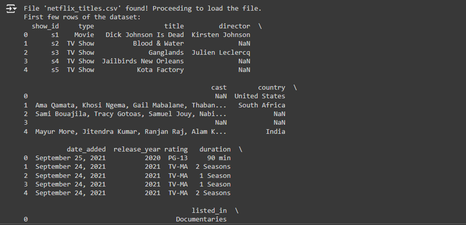
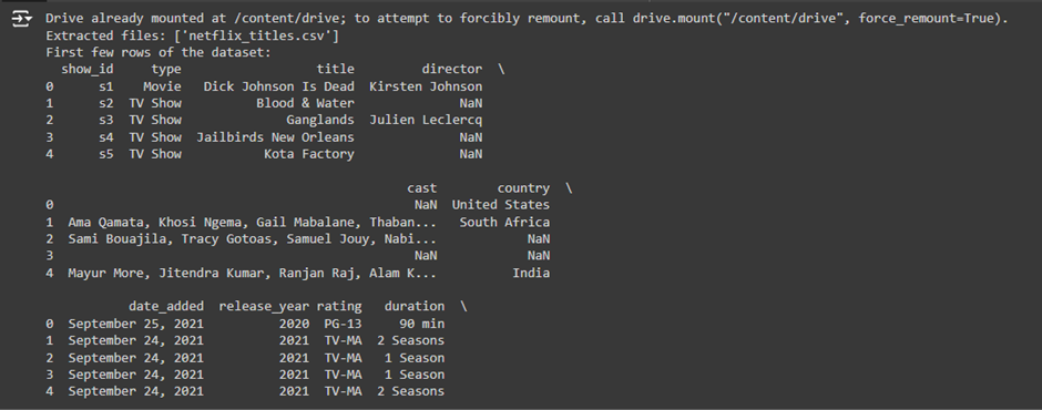
4. Display the first few rows of the data

print(data.head())

Purpose: This line prints the first few rows of the loaded DataFrame to verify that the data was loaded successfully.

• data.head(): This function returns the first 5 rows of the DataFrame by default. It is a quick way to inspect the data and ensure it is loaded correctly.
• Why It’s Important: This step confirms that the CSV file was read correctly. It helps you see if the data has been loaded as expected, whether the columns are named correctly, and if it is properly structured.

1. Create the ‘clicked’ target column

data[‘clicked’] = data[‘release_year’].apply(lambda x: 1 if x > 2015 else 0)

Purpose: This step creates a new column called ‘clicked’ in the dataset. The idea here is to simulate user interaction by assuming users are likelier to click on content released after 2015.

How It Works: The .apply() function is used to apply a custom function to the release_year column. For each entry:

·         If the release year is greater than 2015, the value in the clicked column is set to 1 (meaning the content was clicked).

·         If the release year is less than or equal to 2015, the value is set to 0 (meaning the content was not clicked).

Example:

• If the release_year is 2018, clicked = 1.
• If the release_year is 2013, clicked = 0.

2. Select relevant features and target variable

X = data[[‘type’, ‘release_year’]] # You can add more features here

y = data[‘clicked’]

Purpose: This step selects the input features (X) and the target variable (y) for the logistic regression model.

• X (Features): In this case, the features are ‘type’ (whether it’s a Movie or TV Show) and ‘release_year’.
• y (Target): The target is the ‘clicked’ column we created in the previous step, representing whether a user clicked on the content.

Example:

• Features (X) might be:
  • type: Movie or TV Show.
  • release_year: The year the content was released.
• Target (y): Whether the user clicked (1) or did not click (0) on the content.

3. Encode categorical features

from sklearn.preprocessing import LabelEncoder

label_encoder = LabelEncoder()

X[‘type’] = label_encoder.fit_transform(X[‘type’])

Purpose: The ‘type’ column is categorical (it has non-numeric values like “Movie” and “TV Show”). Machine learning models like logistic regression require numeric values, so we use label encoding to convert the categories into numbers.

• Movie = 1
• TV Show = 0

How It Works:

LabelEncoder(): This transforms the categorical values (Movie and TV Show) into numerical values.

Example:

• A row with type = “Movie” will be converted to 1.
• A row with type = “TV Show” will be converted to 0.

4. Split the data into training and testing sets

from sklearn.model_selection import train_test_split

X_train, X_test, y_train, y_test = train_test_split(X, y, test_size=0.2, random_state=42)

How It Works:

train_test_split(X, y, test_size=0.2):

·         X_train and y_train are the training data and labels.

·         X_test and y_test are the testing data and labels.

·         The test_size=0.2 argument means 20% of the data will be used for testing, and 80% for training.

·         random_state=42: Ensures the same split each time you run the code for consistency in results.

Example:

• If there are 1000 data points, 800 will be used for training and 200 for testing.

5. Train the logistic regression model

model = LogisticRegression()

model.fit(X_train, y_train)

Purpose: This step initializes and trains the logistic regression model using the training data.

• LogisticRegression(): Creates an instance of the logistic regression model.
• model.fit(X_train, y_train): Trains the model on the training data (X_train) and the corresponding labels (y_train).

How It Works:

• The logistic regression algorithm looks at the relationship between the features (type and release_year) and the target variable (clicked or not clicked) to learn a model that can predict clicks for new data.

Example:

• The model will learn that newer content (after 2015) and movies are more likely to be clicked based on the training data.

6. Make predictions

y_pred = model.predict(X_test)

Purpose: This step uses the trained model to predict the test data.

• model.predict(X_test): This function uses the features in the test set (X_test) to predict whether users will click on the content (1) or not (0).

How It Works:

• The model takes the X_test data (not used during training) and makes predictions using the learned relationships from the training data.

Example:

• For a test data point where release_year = 2018 and type = “Movie”, the model might predict clicked = 1 (user clicked).

7. Evaluate the model

7.1. Calculate the accuracy

print(“Accuracy:”, accuracy_score(y_test, y_pred))

Purpose: This step calculates the model’s accuracy, which tells you the proportion of correct predictions.

• accuracy_score(y_test, y_pred): Compares the true labels (y_test) with the predicted labels (y_pred) and calculates the percentage of correct predictions.

Example:

• If the model correctly predicts 90 out of 100 test cases, the accuracy will be 90%.

7.2. Display the confusion matrix

print(“Confusion Matrix:”)

print(confusion_matrix(y_test, y_pred))

Purpose: The confusion matrix shows how many true positives, true negatives, false positives, and false negatives the model made.

• True Positive (TP): Correctly predicted a click (clicked = 1).
• True Negative (TN): Correctly predicted no click (clicked = 0).
• False Positive (FP): Incorrectly predicted a click (predicted clicked = 1, but actual was 0).
• False Negative (FN): Incorrectly predicted no click (predicted clicked = 0, but actual was 1).

Example:

A confusion matrix of:

[[50, 10],

[5, 35]]

means:

• 50 true negatives, 35 true positives.
• 10 false positives, 5 false negatives.

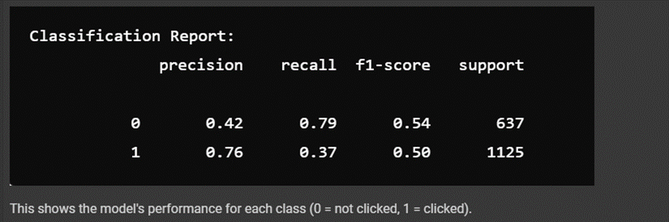
7.3. Display the classification report

print(“Classification Report:”)

print(classification_report(y_test, y_pred))

Purpose: The classification report provides more detailed metrics, including:

• Precision: The proportion of true positive predictions out of all positive predictions.
• Recall: The proportion of actual positive cases that were correctly predicted.
• F1-Score: A balanced metric that combines precision and recall.

Example:

A classification report might show:

Code 1: Netflix Dataset for Predicting User Engagement (Click-Through Prediction)

Purpose:

• Based on the Netflix dataset, this code predicts user engagement (whether a user is likely to click on or interact with content). It uses logistic regression to predict whether content will be “clicked” based on its release year and type (TV Show or Movie).

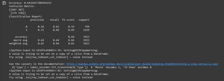
Explaining the Output in Detail:

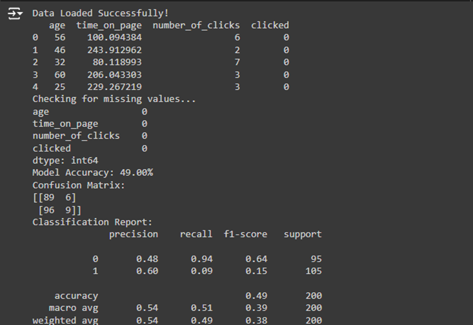
1. Model Accuracy: 0.6432657306292252 (64%)%

·         What It Means: The model correctly predicted whether content would be clicked or not 64% of the time. This means that the model’s overall accuracy is 64%. While this is above random guessing (50% in a binary classification problem like this), it suggests room for improvement.

·         Interpretation: The model is doing moderately well but isn’t perfect. A 64% accuracy shows that the model is making correct and incorrect predictions, and we need to investigate its performance further.

2. Confusion Matrix:

[[487 307]

[379 750]]

What It Is: A confusion matrix provides insight into how well the model performs on each class (in this case, predicting whether content will be clicked or not clicked).

• 487 (True Negatives): The model correctly predicted “no clicks” 487 times.
• 307 (False Positives): The model predicted “clicks” when it should have predicted “no clicks” 307 times.
• 379 (False Negatives): The model predicted “no clicks” when it should have predicted “clicks” 379 times.
• 750 (True Positives): The model correctly predicted “clicks” 750 times.

Interpretation:

·         The model is reasonably good at identifying “clicks” (750 correct predictions) but still misses quite a few (379 times it predicted no clicks when clicks happened).

·         t is also reasonably good at predicting “no clicks” (487 correct predictions) but sometimes incorrectly predicts a click (307 times).

3. Classification Report:

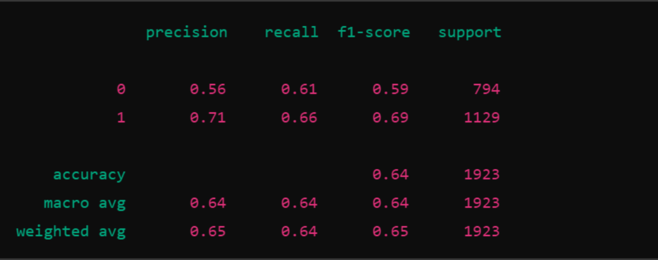
Precision: This tells you how many positive predictions (clicks) were correct.

·         0 (No Clicks): 0.56—The model predicted “no clicks” 56% of the time.

·         1 (Clicks): 0.71 – Out of all the times the model predicted “clicks”, it was correct 71% of the time.

Recall: This tells you how many of the actual instances of each class were correctly identified.

·         0 (No Clicks): 0.61 – The model identified 61% of actual “no clicks”.

·         1 (Clicks): 0.66 – The model identified 66% of actual “clicks”.

F1-Score is the harmonic mean of precision and recall, balancing both metrics.

·         0 (No Clicks): 0.59—The F1-Score balances precision and recall, overall measuring how well the model performs for “no clicks.”

·         1 (Clicks): 0.69 – F1-Score for “clicks” is higher, meaning the model performs better at predicting clicks than no clicks.

Support:

• The support indicates the number of actual examples in each class (794 for “no clicks” and 1129 for “clicks”).

Interpretation:

·         The model has a higher precision and recall for predicting “clicks” (class 1) than for predicting “no clicks” (class 0). This means the model is better at identifying content users will click on but still misses many clicks (as shown by the 66% recall for clicks).

·         The performance for “no clicks” is lower, with the model missing a significant portion of cases where users don’t click (precision of 56% and recall of 61%).

·         Macro Avg: This is the average of precision, recall, and F1-score across both classes, treating them equally. The low values (0.32 for precision) show that the model is unbalanced.

·         Weighted Avg: This considers the number of instances in each class and gives a weighted average. This metric tells you the model is heavily biased toward predicting clicks overall.

---

1. Accuracy (accuracy = 0.64):

·         Definition: Accuracy is the percentage of correct predictions out of all predictions made.

·         Explanation: The model’s accuracy is 64%, which means that out of 1,923 total predictions, approximately 64% were correct. This tells us how often the model gets the overall prediction right (whether it’s predicting “click” or “no click”).

·         Use: Accuracy is a simple metric to evaluate the overall performance, but it can be misleading if the dataset is imbalanced. For example, if 90% of the content were “no clicks”, a model that predicts “no click” 100% of the time would still have high accuracy, even though it fails to predict “clicks.”

2. Macro Average (macro avg):

Definition: Macro average calculates the metric (precision, recall, and F1-score) for each class (in this case, “click” and “no click”) separately and then takes the average.

Explanation:

·         Precision (0.64): On average, the model correctly predicts 64% of the times when it says something will happen (whether predicting clicks or no clicks)

·         Recall (0.64): On average, the model correctly identifies 64% of the actual occurrences for both clicks and no clicks.

·         F1-score (0.64): The F1-score is the harmonic mean of precision and recall, balancing the trade-off between these metrics.

Use: Macro average gives equal importance to both classes (“click” and “no click”) by calculating metrics individually for each class and averaging them. This is useful if you care equally about predicting both outcomes, but it can underestimate performance on imbalanced datasets.

3. Weighted Average (weighted avg):

Definition: The weighted average considers the class imbalance by weighting the metrics based on the number of instances in each class.

Explanation:

·         Precision (0.65): The model correctly predicts 65% of the times it says something will happen, giving more weight to the class that appears more frequently (e.g., more “no clicks”).

·         Recall (0.64): The model correctly identifies 64% of actual occurrences, with the calculation weighted by the number of examples for each class.

·         F1-score (0.65): This weighted F1-score is a balanced measure, considering both precision and recall, while accounting for the number of examples in each class.

Use: Weighted average is useful when your dataset is imbalanced because it accounts for the fact that one class might have more examples than the other. This gives you a more realistic picture of how the model performs overall.

---

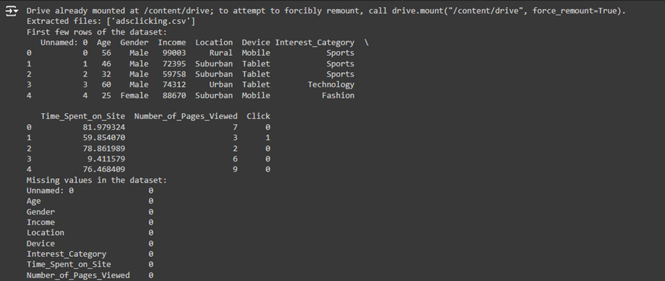
Code 2: Ad Click Prediction (Predicting Ad Engagement)

Purpose:

• This code predicts whether a user will click on an advertisement based on various user and behavior features. It uses logistic regression to predict ad engagement from an Ad Click dataset.

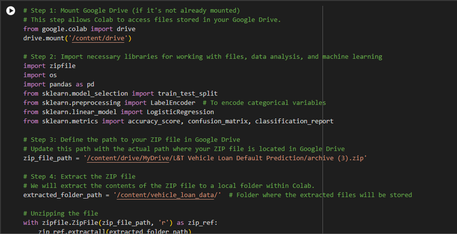
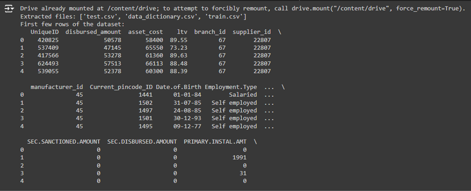
Code 3: L&T Vehicle Loan Default Prediction (Predicting Loan Default)

Purpose:

• This code aims to predict whether a customer will default on a vehicle loan based on their financial data. Logistic regression is used to forecast the probability of loan default based on the L&T Vehicle Loan dataset.

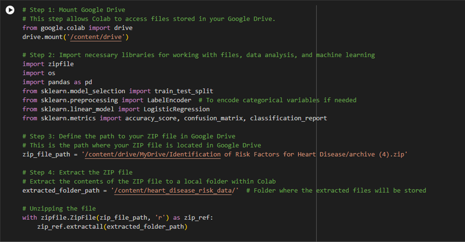
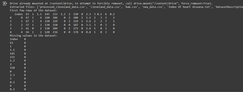
Code 4: Heart Disease Risk Prediction (Predicting Risk of Heart Disease)

Purpose:

• This code predicts a patient’s risk of developing heart disease based on various medical factors. It utilizes logistic regression to classify patients as either likely to have heart disease (1) or not (0) based on the dataset from heart disease studies.

Are the Logistic Regression Codes the Same for Every Field?

Logistic regression generally follows the same core structure regardless of the field. The core steps involve:

·         Data Preprocessing (Handling missing values, encoding categorical variables, selecting features)

·         Splitting the Data (Training and testing sets)

·         Model Training (Training the logistic regression model)

·         Making Predictions (Using the model to make predictions on the test data)

·         Evaluating the Model (Using accuracy, confusion matrix, classification report, etc.)

These steps are the same across different marketing, finance, healthcare, or e-commerce domains.

However, the code has minor differences based on the nature of the data and the problem being solved. Let me explain:

Common Steps Across All Codes:

1. Mounting Google Drive:

• All codes start by mounting Google Drive to access the dataset stored there.

2. Loading the Dataset:

• The datasets are read using pandas and stored in a DataFrame. The only difference is the specific dataset being used, but the process of loading data is identical.

3. Data Preprocessing:

Preprocessing is similar across codes:

• Handling Missing Values: Missing data is handled by filling in values (like mode/median) or dropping missing rows.
• Encoding Categorical Variables: Category variables (like Gender, Device, Employment. Type, etc.) are encoded into numerical values using label encoding. This step is essential for logistic regression and is present in all codes.

4. Splitting the Data:

• All codes use train_test_split to divide the dataset into training (80%) and testing (20%) sets. This step is identical in format and purpose across all the codes.

5. Training the Logistic Regression Model:

• The logistic regression model is trained using LogisticRegression() in all codes. The training process is the same regardless of whether you are predicting ad clicks, loan defaults, or heart disease.

6. Making Predictions:

• After the model is trained, it is used to make predictions on the test set in all codes using the .predict() method.

7. Evaluating the Model:

• The evaluation process is identical across all codes. The accuracy matrix, confusion matrix, and classification report assess the model’s performance. This part of the code is the same in every instance.

---

keyboard_arrow_down

Differences in the Codes:

While the steps and structure of logistic regression are the same, the differences arise from the nature of the dataset and the specific problem being solved. These differences include:

1. Dataset and Features:

Each code uses a different dataset (Netflix, Ad Click, Loan Default, Heart Disease), and therefore the features selected for prediction are different:

·         In the Netflix code, features like type and release_year are used.

·         In the Ad Click code, features like Age, Gender, Device, and Time_Spent_on_Site are used.

· financial features like disbursed_amount, ltv, and PERFORM_CNS are in the Loan Default code.SCORE is used.

· The Heart Disease code uses medical features like age, cholesterol, and blood pressure.

2. Target Variable: 

The target variable (what you’re predicting) is different for each field:

• Netflix: clicked (whether the content was clicked or not)
• Ad Click: Click (whether the user clicked the ad or not)
• Loan Default: loan_default (whether the loan was defaulted or not)
• Heart Disease: 6 (whether the patient has heart disease or not)

3. Handling Categorical Variables:

Depending on the dataset, different categorical variables are encoded. For example:

• In the Ad Click dataset, Gender, Location, and Device are encoded.
• In the Loan Default dataset, Employment.Type is encoded.
• The Netflix dataset encodes the type (Movie or TV Show). Each dataset has different columns that need encoding based on the problem domain.

4. Missing Values:

• Each dataset might have different missing values to handle. In the Loan Default dataset, we fill missing values in the Employment.Type column, while there might be all values in other datasets.

Explanation of the Output:

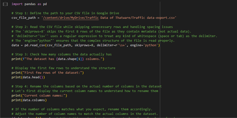
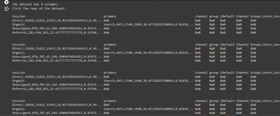
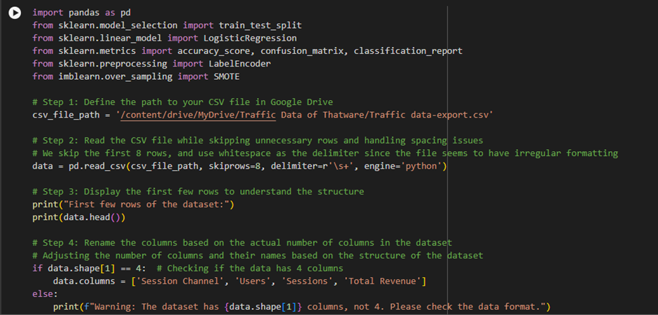
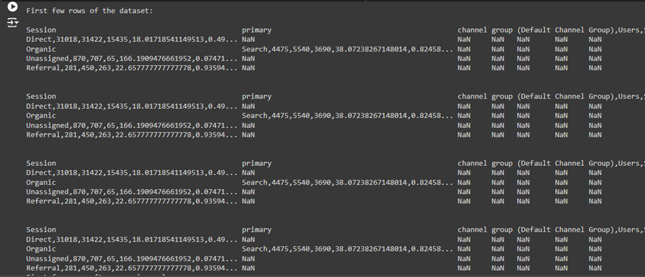
Dataset Overview:

• The dataset appears to have columns like “Session Channel,” “Users,” “Sessions,” and “Total Revenue,” which are supposed to contain information about the website’s traffic and whether it generated revenue or not.

Data Cleaning:

8 We converted the Total Revenue column to numeric and created a binary target variable called Revenue_Flag, which is 1 if the revenue is greater than 0 and 0 otherwise. This variable is the target for the logistic regression model to predict whether a session will generate revenue.

Key Issue:

·         The target variable Revenue_Flag only contains one class (in this case, 0s, meaning there were no sessions that generated revenue).

·         The error message “Error: The target variable ‘Revenue_Flag’ contains only one class” is crucial here. Logistic regression and other machine learning models need at least two classes (like “revenue” and “no revenue”) to learn from and make predictions. Since there is no variability in the target variable (only one class is present), the model cannot function as intended.

What This Means:

·         No Revenue Recorded: The fact that Revenue_Flag contains only 0s means that none of the sessions in the dataset generated any revenue. This could either be an issue with the data itself (e.g., incomplete data collection, missing revenue information) or it could reflect a genuine situation where the website did not generate any revenue from its traffic.

·         Model Cannot Learn: Logistic regression is a classification model that relies on class differences to learn and make predictions. If there is only one class (e.g., “no revenue”), the model has nothing to compare, so it cannot be trained.

---