SUPERCHARGE YOUR ONLINE VISIBILITY! CONTACT US AND LET’S ACHIEVE EXCELLENCE TOGETHER!

This project delivers a structured analytical system designed to evaluate how well a page balances information depth, conceptual richness, and readability flow. The analysis operates at both the section level and page level, using advanced NLP, linguistic metrics, and semantic modelling to detect areas where content is either overloaded with information or lacking sufficient depth.

The system builds a detailed content profile by extracting webpage text, segmenting it into meaningful sections, and computing multiple density- and readability-related features. These include concept compression, information load, semantic complexity, long-sentence ratios, passive voice prevalence, readability friction, and overall linguistic weight. Through these measurements, each section is assigned a balance score that classifies it as over-dense, balanced, or under-dense.

A calibrated thresholding approach ensures that density classification adapts to the global characteristics of each page set. This reduces false positives and enables more meaningful interpretation across varied content styles.

The resulting insights highlight how information is distributed, whether conceptual load is consistent, and which areas may require structural, linguistic, or semantic improvement. The system also includes multiple visualization modules—such as distribution charts, section-level trend analysis, and page-level radar plots—to make patterns easily interpretable.

Overall, the Content Density Equilibrium Analyzer provides a comprehensive, data-driven understanding of how content density, clarity, and reading effort interact across a page. This helps ensure that content maintains both richness and accessibility, supporting stronger engagement, clarity of communication, and improved content performance across search and user experience contexts.

---

Project Purpose

The primary purpose of the Content Density Equilibrium Analyzer is to provide a structured, data-driven framework for understanding whether page content maintains an effective balance between conceptual depth and readability ease. In practical terms, the system identifies how efficiently information is delivered, how evenly conceptual load is distributed, and where linguistic friction increases or decreases reader comprehension.

Modern SEO and content workflows frequently suffer from two opposing issues:

1. Over-dense sections that compress too many ideas, increasing cognitive load and reducing clarity.
2. Under-dense sections that contain insufficient semantic depth, lowering informational value and topical strength.

This project addresses both issues by integrating semantic modelling, linguistic measurement, and readability evaluation into a unified diagnostic process. The system quantifies density and clarity through multiple perspectives—concept coverage, information packaging, sentence structure, vocabulary diversity, and semantic variation.

The purpose is not only to measure density but to explain why certain sections deviate from the ideal balance. Each section receives an interpretable balance score, classification label, and a reasoning summary that explains its conceptual or linguistic issues in a way that supports actionable refinement.

The ultimate goal is to enable systematic improvement of content structure, clarity, and topical delivery. By revealing over-loaded or under-developed areas, the tool helps create content that is both rich in information and smooth to read, promoting stronger user engagement, better comprehension, and improved alignment with modern quality-driven search evaluation standards.

---

Project’s Key Topics Explanation and Understanding

A balanced content experience depends on how effectively a page distributes information, concepts, and linguistic complexity. The Content Density Equilibrium Analyzer evaluates this balance by examining the interplay between semantic depth and readability. The following key topics outline the foundational concepts assessed throughout the project.

Content Density

Content density describes how much meaningful information is packed into a given span of text. High density typically indicates a large concentration of concepts, data, or complex statements within a small section. Low density, on the other hand, reflects minimal conceptual presence despite occupying space.

Density is influenced by three primary elements:

• Concept volume (how many distinct ideas appear)
• Information packaging style (how tightly ideas are grouped)
• Sentence structure complexity (how hard text is to digest)

Sections that compress too many ideas become cognitively demanding, while sections with too few ideas feel shallow or redundant. This project measures density with multiple features to capture both conditions accurately.

Information Depth

Information depth reflects how substantively a section contributes to the overall theme or topic. Depth is not merely about word count; it is about the richness, clarity, and distinctiveness of the ideas provided.

Depth-related measurements include:

• Concept diversity
• Concept entropy
• Semantic variance
• How effectively ideas build on one another

When information depth is too low, a section may appear vague or superficial. When too high, it may overwhelm readers. The project quantifies this depth to understand whether the content meaningfully advances topic understanding.

Readability

Readability describes how easily a human reader can process the language used in a section. Even highly informative content can fail if readability drops below a certain threshold.

Several linguistic signals influence readability:

• Frequency of long or complex sentences
• Passive voice usage
• Vocabulary variation
• Readability indices such as SMOG

The project integrates these signals to assess how smoothly a reader can absorb information. Readability is interpreted alongside semantic features to understand whether linguistic load contributes to over-density or under-density.

Balance Between Depth and Readability

The central principle of this project is the equilibrium point between semantic richness and linguistic simplicity. A balanced section:

• Provides enough conceptual depth to be meaningful
• Distributes ideas without compressing them excessively
• Maintains a reading flow that does not create friction
• Avoids padding or filler content that reduces informational value

The system evaluates balance using a unified score that merges density features, semantic depth indicators, and readability load. This equilibrium score is the foundation for classifying each section as over-dense, balanced, or under-dense.

Over-Dense Sections

An over-dense section concentrates too many ideas, technical elements, or complex structures into too little space. This creates cognitive strain and disrupts clarity.

Typical characteristics include:

• High conceptual compression
• Dense semantic clusters
• Elevated complexity and readability friction
• Heavy informational load

Over-dense sections often require restructuring to improve clarity and pacing without losing informational value.

Under-Dense Sections

An under-dense section contributes limited conceptual or informational value relative to its length. Such sections weaken topic delivery and reduce the perceived depth of a page.

Signals commonly associated with under-density include:

• Low concept diversity
• Minimal semantic variation
• Repetitive or generic statements
• Unused space where more actionable information could exist

Under-dense areas usually require enrichment through clearer ideas, deeper explanation, or more practical insights.

Conceptual Load vs. Linguistic Load

Two different types of “load” influence density:

ceptual Load

The amount and complexity of ideas presented. High conceptual load increases cognitive effort, especially when concepts are tightly packed.

guistic Load

The difficulty imposed by language itself. Text may be grammatically correct yet still hard to read due to long sentences, vocabulary density, or structural complexity.

The analyzer evaluates both loads independently and jointly, allowing precise identification of whether a section is dense due to the content itself, the writing style, or a combination of both.

Semantic Variation and Concept Distribution

Healthy content demonstrates variation in ideas and terminology without redundancy. Semantic variation indicates how diversified and contextually relevant the concepts are across a section.

Key semantic aspects include:

• Distribution of concepts throughout the section
• Diversity of meaningful terms
• Relationships among concepts
• Degree of repetition versus new information

These metrics help determine whether a section advances the topic or merely rephrases the same points.

Balance Score and Classification Framework

At the core of the analyzer is a balance score that combines multiple categories of features:

• Over-density indicators
• Under-density indicators
• Readability signals
• Semantic depth metrics
• Information load

The resulting score is interpreted through calibrated thresholds to classify each section as:

• Over-dense
• Balanced
• Under-dense

Each classification is paired with an interpretation that explains the underlying causes in practical terms.

---

keyboard_arrow_down

Q&A: Understanding Project Value and Importance

What specific problem does the Content Density Equilibrium Analyzer solve?

Webpages often suffer from imbalance—either by overloading readers with dense, complex information or by presenting content that is shallow and lacks substantive value. This imbalance weakens comprehension, disrupts reading flow, and reduces topical satisfaction. The analyzer identifies these imbalances in a structured, measurable way by evaluating how ideas, complexity, and readability interact within each section. Instead of relying on surface-level metrics like word count, the system assesses semantic depth, information load, and linguistic friction simultaneously. This comprehensive approach makes the resulting insights far more actionable than traditional content audits.

Why is balancing semantic depth and readability important for high-performing content?

High-performing content must communicate meaningful ideas while remaining accessible. When semantic depth is high but readability is poor, readers experience cognitive overload and disengage. When readability is smooth but semantic depth is low, the page appears vague or unhelpful. Balancing both ensures that a page delivers high informational value without making users work too hard to understand it. This equilibrium supports stronger engagement signals, better user experience, and more persuasive content pathways.

How does this system add value beyond regular SEO content audits?

Traditional audits typically focus on keyword placement, visibility factors, and structural elements. However, they rarely analyze the quality of idea distribution within the content itself. This analyzer evaluates the internal balance of meaning across a page. It highlights:

• Where ideas are compressed too tightly
• Where content lacks depth
• How complexity affects readability
• How well semantic variety supports topical coverage

This type of analysis fills a long-standing gap in content quality evaluation, supporting more strategic optimization decisions that go beyond keywords and formatting.

What makes the analyzer different from generic readability checkers or NLP scoring tools?

Generic readability tools assess surface-level linguistic difficulty but ignore meaning. General NLP scoring tools may detect sentiment or topic presence but do not evaluate how well ideas are structured within a section. This analyzer combines both worlds by interpreting conceptual load, semantic diversity, information packaging, and linguistic friction together. Instead of rating readability alone, it determines whether the meaning and the structure reinforce or conflict with each other—something traditional tools cannot measure.

How can content teams benefit from detecting over-dense sections?

Over-dense sections often contain valuable insights but present them in a way that overwhelms readers. By isolating these sections, the analyzer reveals precisely where clarity can be improved without sacrificing depth. Rewriting guidance becomes easier because the system shows whether complexity is driven by excessive ideas, difficult language, or both. This enables more strategic content refinement, improves user engagement, and helps retain readers through information-heavy segments.

How does identifying under-dense sections strengthen topic authority?

Under-dense sections dilute topical depth and reduce perceived expertise. By highlighting these areas, the analyzer reveals where additional explanation, examples, or conceptual expansion will strengthen the page. Rather than guessing which parts feel shallow, teams receive a data-backed indication of where depth is currently insufficient and needs enhancement to boost completeness and authority.

Why is section-level analysis more practical than page-level scoring alone?

A page-level score provides an overall impression, but it hides structural weaknesses inside the content. Pages with strong overall performance can still contain problematic sections that disrupt flow or weaken topic delivery. Section-level analysis pinpoints these areas with precision. This empowers content teams to make targeted improvements, reducing the time and effort required to diagnose issues manually.

How does the analyzer ensure that findings remain aligned with real reading experiences?

The system evaluates both semantic and linguistic elements, reflecting how real readers interpret content. High conceptual load, dense clusters of ideas, or difficult sentence structures produce friction that readers immediately feel. By modeling these signals, the analyzer mirrors genuine user experience rather than relying on superficial indicators. This alignment makes its insights relevant for optimizing readability, depth, and clarity in ways that directly affect audience perception.

Can the analyzer help maintain consistency across multi-section or long-form content?

Yes. Long-form content often varies in density as topics shift, contributors differ, or sections evolve over time. The analyzer provides a unified density baseline against which all sections can be compared. This helps maintain consistent pacing, conceptual depth, and readability throughout the page. The resulting uniformity strengthens narrative flow, improves comprehension, and enhances the professional feel of the content.

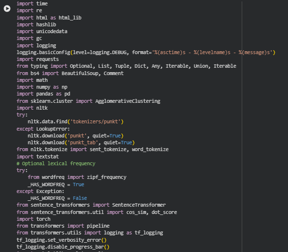
Libraries Used

time

The time library provides basic time-handling utilities such as timestamps and sleep functions, commonly used for performance measurement or pacing operations. It is a lightweight standard library module frequently applied in automation and data processing workflows.

Within this project, time is used during certain stages of data processing to track procedural duration, manage pacing when handling multiple URLs, and assist in debugging performance bottlenecks. This helps ensure stable execution during large-scale content evaluation.

re

The re module implements regular expressions, enabling structured text search, pattern-based extraction, and flexible string manipulation. It is a core tool for any natural language or web data processing task where precise matching or cleaning is required.

In this project, re supports HTML cleanup, text normalization, label trimming for visualizations, and structural extraction of content segments. It ensures consistency in preprocessing and enables accurate parsing of noisy or variable webpage content.

html (html_lib)

The built-in html module provides utilities to handle HTML entities, escape characters, and perform conversions between encoded and decoded text representations. It is particularly relevant when processing raw text extracted from web pages.

Here, html_lib assists in unescaping HTML entities from webpage content, ensuring that the analyzed text reflects human-readable content rather than encoded artifacts. This improves accuracy in linguistic and semantic feature computation.

hashlib

hashlib offers hashing algorithms used to generate unique, reproducible identifiers based on input content. It is widely used for cryptographic hashing, deduplication, and lightweight identity generation.

In this project, it generates unique, stable section identifiers based on section text. While these identifiers are not shown to end users, they provide reliable internal references for tracking sections across processing stages.

unicodedata

The unicodedata module supports Unicode text normalization, character category lookups, and consistent processing of multilingual content. This is essential for text-intensive systems that rely on character-level consistency.

Here, it ensures normalized text representation before tokenization and semantic analysis. By removing inconsistencies such as mixed encodings or combined characters, the project maintains accurate and uniform linguistic measurement.

gc (garbage collector)

The gc module controls Python’s garbage collection, allowing explicit memory cleanup and inspection. It is particularly helpful in large-scale NLP pipelines where memory spikes may occur.

This project uses gc to release unused objects during multi-URL processing, preventing memory buildup when generating embeddings or handling large HTML payloads. This maintains stable performance across long-running sessions.

logging

The logging library provides configurable logging utilities for debugging and monitoring code execution. It is preferred over print statements for production-grade systems due to its flexibility and structured formatting.

Logging is integrated into this project to record processing steps, detect anomalies in data extraction, and support traceability during multi-stage NLP operations. This supports reliability and debugging without interrupting the analytic flow.

requests

The requests library is the industry-standard HTTP client for fetching web content in Python. It simplifies sending requests and managing responses across the web.

This project uses requests to fetch webpage HTML content directly from URLs. It ensures stable retrieval, handles network errors gracefully, and provides a reliable interface for feeding page content into the content-density pipeline.

typing

The typing module provides type annotations that improve readability, reduce errors, and support modern development tools and IDEs.

In the project, typing clarifies expected data structures such as lists of sections, dictionaries of metrics, or optional arguments. This maintains code quality and structural consistency across the entire pipeline.

BeautifulSoup (bs4)

BeautifulSoup is a widely used HTML parsing library that allows structured navigation, cleaning, and extraction of content from web pages.

Here, it extracts readable text from HTML by removing scripts, styles, comments, and structural noise. This ensures that semantic and linguistic analysis focuses solely on meaningful content rather than irrelevant markup.

math

The math library provides mathematical functions and constants used in calculations such as logarithms, trigonometry, and rounding.

This project uses math for geometric and statistical computations, including radar chart angles and score normalization. It enables precise numerical handling within the visualization and density scoring logic.

numpy (np)

NumPy is a foundational numerical computing library offering efficient array operations, mathematical functions, and linear algebra routines.

In this project, NumPy powers vector-based computations, such as embedding norms, density ratios, and matrix transformations. It ensures fast processing when generating semantic metrics and producing aggregated section statistics.

pandas (pd)

Pandas is the standard library for structured data analysis in Python. It supports dataframes, indexing, aggregation, and tabular manipulation.

The project converts section-level and page-level metrics into pandas dataframes for visualization, aggregation, and intermediate organization. This enables efficient plotting, correlation evaluation, and cross-page comparison.

sklearn.cluster.AgglomerativeClustering

AgglomerativeClustering is a hierarchical clustering method used to group items based on similarity. It is often used in NLP workflows to cluster sentences, topics, or embeddings.

Here, it groups semantically similar sentences to support redundancy detection, semantic mass distribution, or topic compactness evaluation. This contributes to downstream density scoring and improves interpretation of conceptual structure.

nltk + punkt tokenizers

NLTK is a classical natural language processing library that provides tokenization, stemming, corpora access, and sentence segmentation.

In this project, NLTK supplies sentence and word tokenizers essential for linguistic metrics such as sentence count, word count, sentence-length distribution, and readability estimates. These foundational metrics feed directly into density scoring.

textstat

Textstat provides a suite of readability formulas such as Flesch Reading Ease, SMOG, and Gunning Fog. These models estimate reading difficulty based on linguistic features.

Here, it computes readability load, long-sentence ratios, and linguistic friction indicators. These scores help determine whether textual complexity contributes to over-density or supports balanced content structure.

wordfreq (optional)

The wordfreq library estimates word frequency using large multilingual corpora. It helps evaluate lexical rarity.

In this project, it optionally enhances lexical richness scoring when available. Rare word usage can signal conceptual depth but may introduce unnecessary friction, influencing overall density classification.

sentence_transformers (SentenceTransformer, cos_sim, dot_score)

sentence_transformers provides state-of-the-art transformer models for embedding text into high-dimensional semantic vectors.

This project uses the model to encode section text for calculating semantic mass, conceptual differentiation, embedding-based complexity metrics, and inter-sentence similarity. These embeddings form the backbone of semantic density scoring.

torch

PyTorch is a deep learning framework used to run transformer models, tensor computations, and GPU-accelerated operations.

It supports the SentenceTransformer encoding process, enabling efficient embedding computation even at scale. Without PyTorch, transformer-based semantic scoring would be significantly slower.

transformers (pipeline)

Hugging Face’s transformers library provides pretrained NLP models for summarization, sentiment, classification, and more.

Here, the sentiment pipeline is used to detect subtle tonal or structural shifts when required. It complements semantic indicators and contributes to the tension score used in density interpretation.

matplotlib.pyplot (plt)

Matplotlib is the foundational plotting library in Python that supports fine-grained, customizable visualizations.

In the project, it renders all major plots—including density distribution, section-level performance, and radar charts. It provides layout control and ensures professional-quality presentation of project results.

seaborn (sns)

Seaborn builds on Matplotlib and provides modern statistical visualizations with enhanced aesthetics and simplicity.

It enables clearer, publication-ready representations of density metrics, comparative distributions, and multi-page trends. Styled plots support intuitive interpretation and make complex data more accessible.

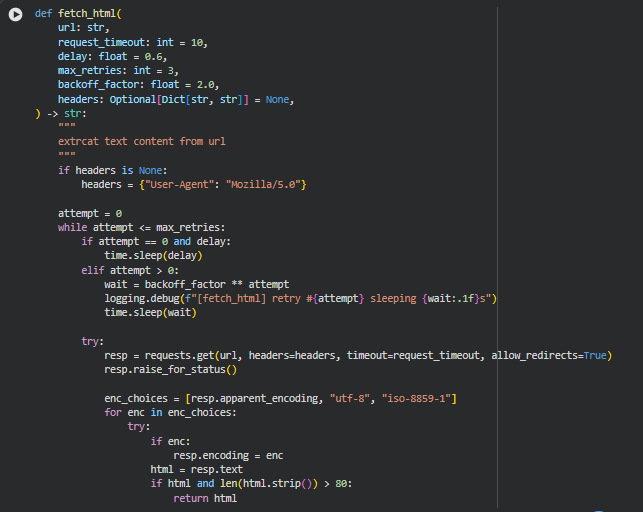
Function: fetch_html

Summary

This function is responsible for retrieving the raw HTML content from a given webpage URL in a stable, fault-tolerant manner. Real-world websites frequently introduce challenges such as slow response times, temporary network drops, redirects, inconsistent character encodings, or incomplete responses. This function is designed to address those challenges through controlled retry logic, flexible encoding handling, adjustable waiting periods, and safety checks that ensure only meaningful HTML content is returned.

Within the project, this function serves as the foundational step of the entire analysis pipeline. Every downstream process—content extraction, structuring, sentence segmentation, embedding generation, and density evaluation—depends on reliable and consistent HTML input. By ensuring robust fetching with retry and backoff mechanisms, the function minimizes disruption during multi-URL analysis and ensures smooth operation even when target sites behave unpredictably.

Key Code Explanations

if headers is None: headers = {“User-Agent”: “Mozilla/5.0”}

A default user agent is applied when none is provided. Many websites block requests that do not resemble standard browser traffic. Using a browser-like user agent helps reduce the chance of being flagged or denied by servers.

Retry Loop:

while attempt <= max_retries:

The function attempts the request multiple times before giving up. This prevents temporary network issues or server delays from causing the entire workflow to fail.

Exponential Backoff:

wait = backoff_factor ** attempt
time.sleep(wait)

When a retry is needed, the waiting time increases exponentially. This mirrors real-world resilient network design, reducing the load on the server and increasing the chance of a successful response after temporary failures.

Encoding Handling:

enc_choices = [resp.apparent_encoding, “utf-8”, “iso-8859-1”]

Webpages frequently use non-standard or incorrectly reported encodings. Trying multiple encoding candidates ensures the returned HTML is readable and not garbled.

HTML Quality Check:

if html and len(html.strip()) > 80:
    return html

Very short or empty responses typically indicate errors, blocked access, or partial loads. This check ensures only meaningful HTML content is accepted for analysis.

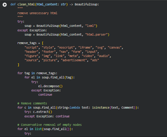
Function: clean_html

Summary

This function transforms the raw HTML into a cleaner and more analysis-ready structure. Webpages often contain large amounts of non-content elements—scripts, styles, navigation panels, ads, tracking tags, media containers, invisible nodes, and comment blocks. These elements provide no semantic value for density assessment, yet they introduce noise that can distort text extraction and downstream computations such as chunking, embedding, and readability scoring.

The function uses BeautifulSoup to parse the HTML and systematically remove irrelevant or disruptive tags. It then clears out HTML comments and prunes empty or placeholder nodes. The result is a purified document tree containing only meaningful textual and structural elements. This cleaned representation ensures that section boundaries, semantic density measures, and content segmentation genuinely reflect the substance of the page rather than clutter or interface artifacts.

Because content density relies heavily on accurate text representation, this cleaning stage directly influences the quality of the final density balancing insights. A well-cleaned HTML structure prevents artificially inflated depth measurements and maintains reliable readability evaluation.

Key Code Explanations

Parser Selection:

soup = BeautifulSoup(html_content, “lxml”)

The function attempts to parse HTML using lxml—a high-performance parser known for speed and accuracy. If unavailable or if parsing fails, it falls back to Python’s built-in “html.parser”, ensuring reliability regardless of environment constraints.

Tag Removal List:

remove_tags = [“script”, “style”, “noscript”, “iframe”, …]

This predefined set includes elements that do not contribute meaningful textual information. Removing them eliminates noise from layouts, advertisements, embedded media, and scripts that may otherwise pollute extracted content.

Iterative Tag Cleanup:

for tag in remove_tags:

    for el in soup.find_all(tag):

        el.decompose()

Each unwanted tag is identified and removed from the document tree. decompose() ensures both the tag and its children are fully discarded, resulting in a lighter, content-centric structure.

Comment Removal:

for c in soup.find_all(string=lambda text: isinstance(text, Comment)):

    c.extract()

HTML comments often contain tracking code, metadata, or developer notes. Removing them ensures only visible and meaningful text remains.

Pruning Empty Nodes:

if not el.get_text(strip=True) and not el.attrs:

    el.decompose()

After major tags are cleared, some nodes become empty shells. This condition removes nodes that have no text and no attributes, preventing clutter during content extraction and section segmentation.

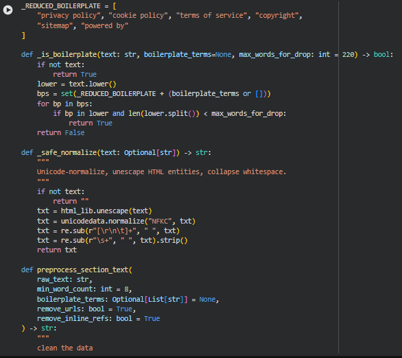
Function: _is_boilerplate

Summary

This helper function identifies and filters out boilerplate text that typically appears on webpages but carries no semantic or analytical value. Examples include footer disclaimers, copyright notices, cookie banners, or generic platform credits. These elements can distort content density calculations by adding low-value text, so removing them ensures the analysis focuses only on meaningful sections of the page.

The function performs lightweight pattern matching on lowercase text and checks whether the size of the text block is small enough to qualify as boilerplate. This avoids accidental removal of large, meaningful sections that happen to contain one of the boilerplate terms.

Key Code Explanations

Boilerplate Set Construction:

bps = set(_REDUCED_BOILERPLATE + (boilerplate_terms or []))

This merges a predefined list of boilerplate fragments with any custom terms provided. Using a set improves lookup efficiency during repeated checks.

Boilerplate Detection Logic:

if bp in lower and len(lower.split()) < max_words_for_drop:

    return True

The text is classified as boilerplate only if it contains a boilerplate phrase and is short enough to be considered non-content. This prevents legitimate long sections from being accidentally removed.

Function: _safe_normalize

Summary

This function ensures all text segments are normalized, clean, and consistent before any linguistic processing occurs. HTML pages often contain irregular spacing, escaped characters, Unicode inconsistencies, and formatting artifacts. The normalization step converts text into a standardized form that improves the reliability of tokenization, semantic embedding, readability calculation, and density measurement.

By performing Unicode normalization, HTML entity decoding, and whitespace cleanup, this function prepares the text so that downstream functions operate on clean and predictable inputs.

Key Code Explanations

Unicode + HTML Cleanup Pipeline:

txt = html_lib.unescape(text)

txt = unicodedata.normalize(“NFKC”, txt

txt = re.sub(r”[\r\n\t]+”, ” “, txt)

txt = re.sub(r”\s+”, ” “, txt).strip()

This sequence performs three essential cleanup steps:

• Converts HTML entities into readable characters.
• Standardizes Unicode formatting for consistency.
• Removes line breaks, tabs, and excess spaces to ensure clean word boundaries.

Function: preprocess_section_text

Summary

This function performs the final cleaning step for each extracted text section before it is analyzed. It applies normalization, removes inline clutter such as URLs and reference markers, filters out boilerplate fragments, and enforces a minimum word count. The goal is to ensure each section fed into the density computation pipeline contains meaningful, interpretable text with minimal noise.

By strengthening the signal-to-noise ratio, this function ensures that semantic embeddings, concept extraction, readability assessment, and density balancing reflect the actual content quality rather than structural residue or irrelevant text blocks.

Key Code Explanations

URL Removal:

text = re.sub(r”https?://\S+|www\.\S+”, ” “, text)

Inline URLs often inflate word counts and introduce irrelevant tokens. This line safely removes them to prevent distortion in readability and density metrics.

Inline Reference Removal:

text = re.sub(r”\[\d+\]|\(\d+\)”, ” “, text)

Academic-style inline references provide no value to density assessment and can interfere with token distribution, so they are stripped.

Boilerplate Filtering:

if _is_boilerplate(text, boilerplate_terms=boilerplate_terms):

    return “”

By integrating the earlier helper function, this step ensures generic non-informational text does not enter the analysis pipeline.

Minimum Length Enforcement:

if len(text.split()) < min_word_count:

    return “”

Very short fragments lack sufficient semantic structure for density evaluation. This condition prevents them from being misinterpreted as meaningful content.

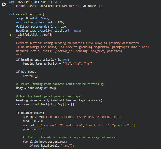
Function: _md5_hex

Summary

This function generates a deterministic and compact hash string for any given text using the MD5 hashing algorithm. The purpose is to create stable identifiers for extracted sections. Webpage content often contains many elements with similar headings or similar text fragments. Instead of relying on raw text or numeric counters—which can collide or change depending on parsing order—this hash-based identifier guarantees uniqueness while keeping the ID short, consistent, and reproducible across runs.

Since section integrity is important for density scoring, semantic embedding, and later result mapping, the use of a stable MD5 hash ensures that each extracted section can be reliably tracked throughout the pipeline.

Key Code Explanations

MD5 Hash Generation:

return hashlib.md5(text.encode(“utf-8”)).hexdigest()

The input text is encoded to UTF-8 bytes, hashed, and converted to a hexadecimal string. This ensures cross-platform stability and avoids issues caused by special characters in raw IDs.

Function: extract_sections

Summary

This function performs structured extraction of meaningful content sections from the cleaned HTML. It uses heading tags as primary boundaries because headings represent natural semantic segmentation created by the page author. When headings are present, the function walks through the document in reading order and constructs section blocks under each heading, merging associated paragraphs and list items.

In cases where a webpage lacks proper headings—common in poorly structured content or dynamically generated pages—the function falls back to grouping sequential paragraphs into blocks of similar size. This ensures robust section extraction even in non-standard HTML layouts.

The function also ensures each section is long enough to be meaningful, assigns a unique ID to each block using the _md5_hex helper, records the heading, raw text, and position, and outputs a list of structured, analyzable sections ready for semantic and density computations.

Key Code Explanations

Heading-Based Section Detection:

heading_nodes = body.find_all(heading_tags_priority)

This detects the presence of any H2, H3, or H4 tags (or any custom hierarchy supplied). If headings exist, the function will use them as natural section dividers.

Iterating Through Document in Reading Order:

for el in body.descendants:

Using descendants preserves the original DOM order, ensuring text flows naturally as the reader would experience it. This prevents fragmentation or misordering of paragraphs.

Heading Boundary Trigger:

if name in heading_tags_priority:

    if len(current[“raw_text”].strip()) >= min_section_chars:

        sec_id_src = f”{current[‘heading’]}_{current[‘position’]}”

        current[“section_id”] = _md5_hex(sec_id_src)

        sections.append(current)

When a new heading is encountered, the previous section is finalized—but only if it has enough text to be meaningful—before starting a new block. This avoids creating empty or trivial sections.

Paragraph Accumulation:

if name in (“p”, “li”):

    txt = _safe_normalize(el.get_text())

    if txt:

        current[“raw_text”] += ” ” + txt

Paragraphs and list items are the main carriers of human-readable text. Each one is cleaned and appended to the current section to keep content coherent.

Fallback Paragraph Grouping:

if len(buffer_words) >= fallback_para_words:

    heading = f”Section {position}”

If no headings exist, the function groups paragraphs until they reach a target word count (default 250 words), then emits a section block. This ensures even poorly structured pages still produce well-formed analytical sections.

Section ID Generation:

sec_id_src = f”{heading}_{position}”

“section_id”: _md5_hex(sec_id_src)

Combining heading text and its order ensures each section receives a unique and stable ID for later analysis.

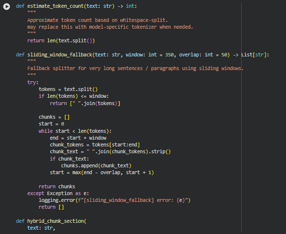
Function: estimate_token_count

Summary

This utility function provides a lightweight approximation of token count by splitting text based on whitespace. Although true tokenization depends on the model in use, this approximation serves as a practical method for chunk sizing, windowing, and sentence grouping without imposing the overhead of loading model-specific tokenizers. It is fast, deterministic, and works consistently across all sections of the pipeline that need quick length estimation.

Because chunk formation, fallback splitting, and size thresholds depend on approximate token lengths rather than exact model tokens, this approach ensures predictable performance and avoids unnecessary complexity.

Function: sliding_window_fallback

Summary

This function generates controlled, overlapping text segments when sentences or paragraph blocks exceed a predefined maximum window size. Very long sentences can break standard semantic chunking workflows, and this fallback ensures that such content is still processed without truncation. It operates by sliding a window across the tokenized text with a configurable overlap, creating coherent chunks that maintain context continuity.

This fallback is essential for pages containing highly compressed or technical text, where extremely long sentences are common. Its behavior ensures that downstream embedding models receive manageable and context-rich inputs.

Key Code Explanations

Sliding window loop:

while start < len(tokens):

    end = start + window

    chunk_tokens = tokens[start:end]

The window moves across the token sequence, capturing fixed-size segments until the end of the text is reached.

Controlled overlap logic:

start = max(end – overlap, start + 1)

This ensures chunks overlap by a defined number of tokens, preserving context between segments and preventing abrupt semantic breaks.

Function: hybrid_chunk_section

Summary

This function performs multi-stage chunking designed specifically for semantic analysis. It first divides the section into sentences, then accumulates them until a threshold is reached, producing balanced, semantically coherent chunks. If a single sentence exceeds the maximum allowed size, the function switches to the sliding window fallback to avoid skipping or breaking the content.

After chunk formation, any chunk that falls below the minimum token threshold is removed to maintain analysis quality. This layered approach ensures that every processed section yields manageable, meaningful units of text suitable for embedding models and density scoring.

Key Code Explanations

Sentence accumulation logic:

current_chunk.append(sent)

token_est = estimate_token_count(” “.join(current_chunk))

Each sentence is added to the current chunk, and its size is estimated. This ensures semantic grouping by respecting sentence boundaries.

Oversized sentence fallback:

if len(current_chunk) == 1:

    chunks.extend(

        sliding_window_fallback(

            current_chunk[0],

            window=max_tokens,

            overlap=sliding_overlap

        )

    )

When a single sentence is too long, the fallback prevents pipeline failure and preserves content richness through controlled segmentation.

Chunk emission before overflow:

final_chunk = ” “.join(current_chunk[:-1]).strip()

If adding a sentence causes the chunk to exceed the token limit, the previous sentences are finalized as one chunk, and the oversized sentence begins a new block.

Final chunk handling:

if estimate_token_count(final_text) > max_tokens:

    chunks.extend(

        sliding_window_fallback(final_text, window=max_tokens, overlap=sliding_overlap)

    )

Any leftover text after sentence traversal is evaluated independently to ensure it fits size constraints, using sliding windows if necessary.

Final filtration:

cleaned = [c.strip() for c in chunks if estimate_token_count(c.strip()) >= min_tokens]

Chunks that are too short to provide meaningful semantic signals are removed to maintain analysis fidelity.

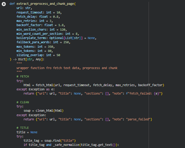
Function: extract_preprocess_and_chunk_page

Summary

This function acts as the full pipeline controller for a single webpage: it fetches the raw HTML from the URL, cleans the HTML structure, extracts meaningful content sections, preprocesses the text, and finally chunks the cleaned text into model-ready units. It is the unifying layer that brings together all lower-level utilities such as HTML fetching, cleaning, section extraction, text preprocessing, and hybrid chunking. Because this is the function clients indirectly benefit from when running the tool, it ensures that even if individual steps fail, the output remains structured, predictable, and useful for downstream ranking analysis, semantic evaluation, or any NLP processing.

The function’s workflow starts by making a robust request to fetch the webpage. If that succeeds, it parses and sanitizes the HTML to remove noise such as scripts, styling, or boilerplate UI components. It then identifies section-level content, cleans the textual data by removing unnecessary or non-informative segments, checks for minimum quality thresholds, and prepares the text for chunking. Once the sections are validated, the chunking system breaks long text into manageable token-bounded segments so that LLM-based models can efficiently process them without losing semantic coherence. Finally, all chunks are organized with metadata such as section position, estimated tokens, and text statistics, resulting in a well-structured and analyzable dataset.

This function is critical because it guarantees consistent structure regardless of HTML variations, content length, or preprocessing edge cases. It centralizes all logic into a clean, deterministic output format essential for the project’s downstream semantic analysis tasks.

The function returns a clean, predictable dictionary object that downstream pipeline components rely upon. The note field only populates in case of errors, making debugging more straightforward.

Function: init_embedding_model

Summary

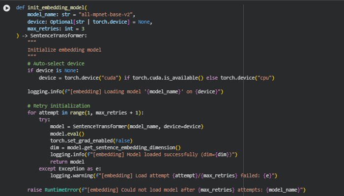
This function loads and initializes the sentence-embedding model used throughout the project. It selects the appropriate compute device (GPU if available, otherwise CPU), loads the specified SentenceTransformer model, and configures it for inference so that no gradients are tracked. A retry mechanism safeguards against temporary model download failures, network instability, or hardware-related initialization errors. The output is a fully ready, inference-optimized embedding model that can quickly transform text chunks into high-quality vector embeddings.

Because embedding generation is central to all downstream semantic tasks—ranking, alignment analysis, depth evaluation—this function ensures the model is always correctly loaded and stable before any text processing begins. Even though the function is short, it plays a crucial role in project robustness.

Key Code Explanations

• Device Auto-Selection

if device is None:

    device = torch.device(“cuda”) if torch.cuda.is_available() else torch.device(“cpu”)

This logic automatically chooses the best computation device. If a GPU is available, embeddings are computed far faster; otherwise, the CPU is used. This ensures the function adapts seamlessly to the environment without requiring manual configuration.

• Model Loading with Retries

for attempt in range(1, max_retries + 1):

    try:

        model = SentenceTransformer(model_name, device=device)

        …

        return model

A retry loop increases reliability. If the first attempt fails—due to transient network issues, download corruption, or device locking—the function tries again. This prevents the entire pipeline from failing prematurely and makes the system resilient for real-world usage.

• Setting the Model for Inference-Only Mode

model.eval()

torch.set_grad_enabled(False)

These two lines disable gradient computation globally for this model. Since the model is only used to generate embeddings (not to train), disabling gradients saves memory, reduces overhead, and increases speed during inference.

Function: compute_readability_metrics

Summary

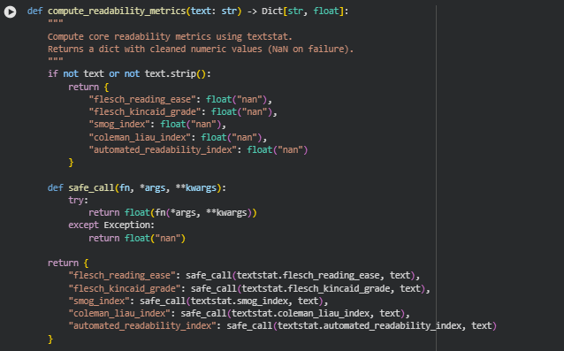
This function calculates core readability scores for a given text using the textstat library. The purpose is to quantify how easy or difficult a section of content is to read, which directly relates to the “readability” aspect of the Semantic Content Density Balancer project. By computing multiple standardized readability metrics, the function provides a multi-dimensional view of text complexity, sentence structure, and cognitive load. Each metric is returned in a dictionary with float values, while handling any errors gracefully by returning NaN for invalid or empty text.

These metrics are later used to compute section-level linguistic load, overall balance, and to support interpretability in section density assessment.

Key Code Explanations

• Safe Metric Computation

def safe_call(fn, *args, **kwargs):

    try:

        return float(fn(*args, **kwargs))

    except Exception:

        return float(“nan”)

The safe_call helper wraps each textstat function call to catch errors caused by unusual input (e.g., very short text, special characters). This guarantees robust metric calculation across diverse web content.

• Computing Multiple Readability Metrics

return {

    “flesch_reading_ease”: safe_call(textstat.flesch_reading_ease, text),

    “flesch_kincaid_grade”: safe_call(textstat.flesch_kincaid_grade, text),

    “smog_index”: safe_call(textstat.smog_index, text),

    “coleman_liau_index”: safe_call(textstat.coleman_liau_index, text),

    “automated_readability_index”: safe_call(textstat.automated_readability_index, text)

}

Here, five widely recognized readability formulas are applied:

• Flesch Reading Ease: Higher values indicate easier text.
• Flesch-Kincaid Grade Level: Represents U.S. school grade level needed to comprehend the text.
• SMOG Index: Estimates years of education required for understanding.
• Coleman-Liau Index: Uses characters per word and sentence length to evaluate readability.
• Automated Readability Index (ARI): Provides another grade-level approximation for text complexity.

By computing multiple metrics, the function gives a balanced assessment of readability that considers both word and sentence complexity.

Function: sentence_level_metrics

Summary

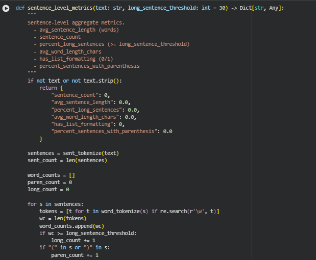
This function calculates sentence-level linguistic metrics to quantify the structural characteristics of a given text. It provides insights into sentence length, complexity, and formatting patterns, which are crucial for understanding readability and cognitive load in content. Metrics include the total number of sentences, average sentence length, the proportion of long sentences, average word length, presence of list-style formatting, and the percentage of sentences containing parentheses. These measurements are important for the Semantic Content Density Balancer project because they directly feed into over-dense and under-dense analysis of sections, complementing semantic and conceptual density calculations.

The results help in assessing linguistic load, sentence complexity, and readability friction, providing a detailed layer of interpretability for each content section.

Key Code Explanations

• Sentence Tokenization and Counting Long Sentences

sentences = sent_tokenize(text)

sent_count = len(sentences)

…

for s in sentences:

    tokens = [t for t in word_tokenize(s) if re.search(r’\w’, t)]

    …

    if “(” in s or “)” in s:

        paren_count += 1

This block performs several critical operations: it splits the text into sentences, counts the words per sentence, identifies sentences exceeding the long_sentence_threshold, and counts sentences containing parentheses. These computations provide direct measures of sentence complexity and structural load.

Average Word Length Calculation

“ words_all = [w for w in word_tokenize(text) if re.search(r’\w’, w)] if words_all: avg_word_len = float(np.mean([len(w) for w in words_all])) `

Here, the function calculates the average number of characters per word, offering insight into lexical density and the potential reading difficulty of the text.

Detection of List Formatting

has_list = 1 if re.search(r'(^|\n)\s*([-*•]|\d+\.)\s+’, text) else 0

This regex detects the presence of common list formats such as bullets (-, *, •) or numbered lists (1., 2.), providing an indication of content organization and visual chunking.

Percentages of Long Sentences and Parentheses

percent_long = (long_count / sent_count) if sent_count else 0.0

percent_paren = (paren_count / sent_count) if sent_count else 0.0

These lines normalize the counts of long sentences and sentences with parentheses to percentages, enabling consistent comparison across sections of varying lengths.

Function: setup_spacy

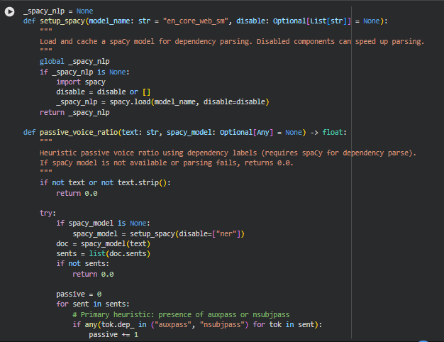
Summary

This function initializes and caches a spaCy NLP model for dependency parsing. It allows selective disabling of pipeline components to speed up processing when full NLP functionality is not required. The cached model ensures that repeated calls to spaCy do not reload the model, improving efficiency for multi-section or multi-page analysis. Dependency parsing is a core step for identifying grammatical structures, particularly for linguistic metrics like passive voice detection.

Function: passive_voice_ratio

Summary

The passive_voice_ratio function calculates the proportion of sentences in a given text that are written in the passive voice. Passive voice sentences tend to increase cognitive load and affect readability, making this metric valuable for assessing linguistic density. The function relies on a spaCy dependency parse to identify passive constructions using both primary and secondary heuristics.

Key Code Explanations

Handling Missing or Empty Text

if not text or not text.strip():

    return 0.0

This ensures robustness by returning a safe default when the input text is empty or only contains whitespace.

Loading or Using Cached spaCy Model

if spacy_model is None:

    spacy_model = setup_spacy(disable=[“ner”])

doc = spacy_model(text)

sents = list(doc.sents)

The function either uses the provided spaCy model or calls setup_spacy to load a cached model with the Named Entity Recognition component disabled for efficiency. The text is then parsed into sentences for further analysis.

Primary Passive Voice Detection

if any(tok.dep_ in (“auxpass”, “nsubjpass”) for tok in sent):

    passive += 1

    continue

This checks for dependency labels auxpass or nsubjpass, which are canonical indicators of passive voice in English, and counts such sentences as passive.

Secondary Heuristic: Be-Aux + Past Participle

for i, tok in enumerate(sent):

    if tok.lemma_.lower() in (“be”, “is”, “was”, “were”, “been”, “being”) and i + 1 < len(sent):

        nxt = sent[i + 1]

        if getattr(nxt, “tag_”, None) == “VBN”:

            passive += 1

            break

This pattern identifies sentences where a form of “be” is immediately followed by a past participle (VBN), which is a common passive voice construction. It serves as a fallback for cases where the dependency parse may not explicitly label a token as passive.

Safe Ratio Calculation

return passive / len(sents)

The function returns the fraction of passive sentences over total sentences, providing a normalized ratio that can be used in density scoring. If spaCy fails or is missing, the function safely returns 0.0 to avoid breaking the pipeline.

Function: lexical_complexity

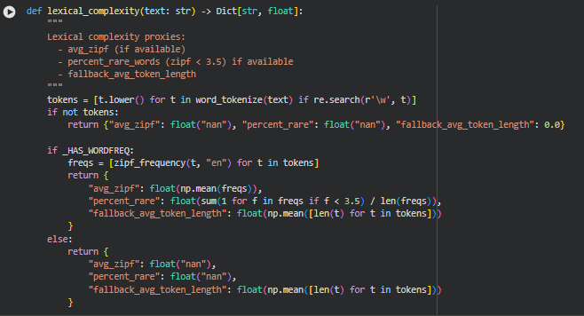
Summary

The lexical_complexity function estimates the lexical richness and difficulty of a text. It uses word-level metrics to quantify how complex or rare the vocabulary is, which directly affects readability and semantic density. When the optional wordfreq library is available, the function computes average Zipf frequency and the percentage of rare words. As a fallback, it calculates average token length to provide a basic approximation of lexical difficulty. These metrics are useful in understanding how challenging a section might be for readers and contribute to the overall density interpretation.

Key Code Explanations

Tokenization and Filtering

tokens = [t.lower() for t in word_tokenize(text) if re.search(r’\w’, t)]

This line splits the text into individual word tokens while filtering out punctuation or non-word symbols. All tokens are converted to lowercase to ensure consistent lexical analysis.

Handling Empty Text

if not tokens:

    return {“avg_zipf”: float(“nan”), “percent_rare”: float(“nan”), “fallback_avg_token_length”: 0.0}

If no valid word tokens are found, the function returns safe default values to avoid downstream errors.

Lexical Metrics Using Word Frequency

if _HAS_WORDFREQ:

    freqs = [zipf_frequency(t, “en”) for t in tokens]

    return {

        “avg_zipf”: float(np.mean(freqs)),

        “percent_rare”: float(sum(1 for f in freqs if f < 3.5) / len(freqs)),

        “fallback_avg_token_length”: float(np.mean([len(t) for t in tokens]))

    }

If the wordfreq library is installed, this block computes the Zipf frequency for each token. Average Zipf frequency reflects overall word commonality, and percent_rare calculates the proportion of rare words (Zipf < 3.5). The fallback average token length is still computed for reference.

Fallback Without Word Frequency

else:

    return {

        “avg_zipf”: float(“nan”),

        “percent_rare”: float(“nan”),

        “fallback_avg_token_length”: float(np.mean([len(t) for t in tokens]))

    }

If wordfreq is unavailable, the function provides NaN for Zipf-based metrics but still returns the average token length, ensuring minimal lexical complexity insight is retained.

Function type_token_ratio

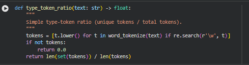
Summary

This function calculates the type-token ratio (TTR) of a given text, which measures lexical diversity. It is computed as the number of unique tokens (types) divided by the total number of tokens. Higher values indicate more varied vocabulary, while lower values suggest repetition. The function tokenizes the text using NLTK, filters non-alphanumeric tokens, and converts all tokens to lowercase to ensure consistency. This metric helps assess content richness and semantic complexity.

Key Code Explanations

Tokenization and normalization

tokens = [t.lower() for t in word_tokenize(text) if re.search(r’\w’, t)]

The text is split into individual word tokens. Tokens that contain no word characters (like punctuation or symbols) are removed. All tokens are converted to lowercase to avoid counting the same word with different cases multiple times. This ensures an accurate count of unique words.

Type-token ratio computation

return len(set(tokens)) / len(tokens)

The unique tokens are identified using set(tokens). Dividing the number of unique tokens by the total token count gives a ratio between 0 and 1, representing the lexical diversity of the text. For empty or whitespace-only text, the function safely returns 0.0.

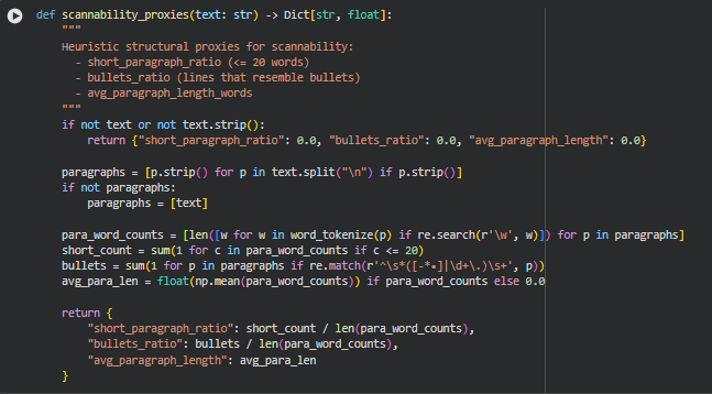
Function scannability_proxies

Summary

This function calculates heuristic structural metrics to estimate the scannability of a text. Scannability reflects how easily a reader can skim through the content. The function considers short paragraphs, bullet-like lines, and average paragraph length. These proxies help determine if the content layout supports quick comprehension, which is critical for web readability and user engagement. For empty or whitespace-only input, it safely returns zeros.

Key Code Explanations

Paragraph extraction and fallback

paragraphs = [p.strip() for p in text.split(“\n”) if p.strip()]

if not paragraphs:

    paragraphs = [text]

The text is split on newline characters to identify paragraphs. Leading and trailing spaces are removed. If no paragraph breaks are detected, the entire text is treated as a single paragraph, ensuring the function can handle unformatted text.

Word count per paragraph

para_word_counts = [len([w for w in word_tokenize(p) if re.search(r’\w’, w)]) for p in paragraphs]

Each paragraph is tokenized using NLTK, counting only alphanumeric tokens. This yields an accurate word count per paragraph, which is used to calculate metrics like short paragraph ratio and average paragraph length.

Short paragraph ratio and bullet detection

short_count = sum(1 for c in para_word_counts if c <= 20)

bullets = sum(1 for p in paragraphs if re.match(r’^\s*([-*•]|\d+\.)\s+’, p))

short_count tracks paragraphs with 20 or fewer words. bullets counts lines resembling lists using a regular expression that matches common bullet symbols or numbered patterns. These proxies reflect quick readability and structured content.

Average paragraph length and final metric computation

avg_para_len = float(np.mean(para_word_counts)) if para_word_counts else 0.0

return {

    “short_paragraph_ratio”: short_count / len(para_word_counts),

    “bullets_ratio”: bullets / len(para_word_counts),

    “avg_paragraph_length”: avg_para_len

}

The mean word count per paragraph is calculated for overall content density. Ratios for short paragraphs and bullets are normalized by the number of paragraphs. These metrics collectively quantify scannability in a concise and interpretable way.

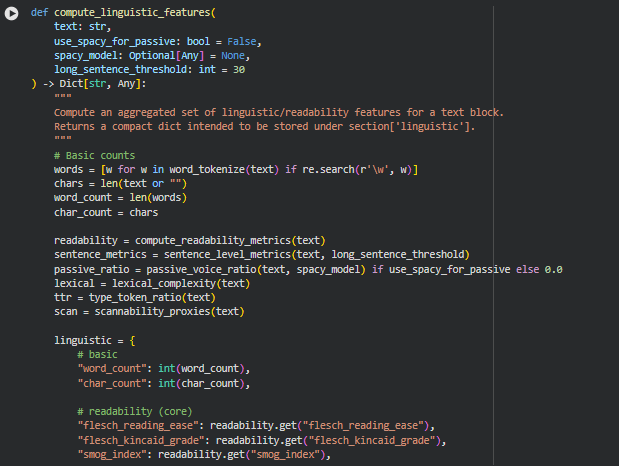
Function compute_linguistic_features

Summary

This function aggregates a comprehensive set of linguistic and readability metrics for a given text block. It is designed to produce a compact dictionary that can be stored under section[‘linguistic’] in the page analysis pipeline. The metrics cover multiple dimensions including basic counts (words, characters), readability (Flesch, SMOG, etc.), sentence-level properties (average length, long sentences), lexical complexity, type-token ratio, scannability, and optionally passive voice ratio. Collectively, these features provide a holistic view of the text’s linguistic profile, which is critical for evaluating content density, readability, and user experience.

Key Code Explanations

Basic word and character counts

words = [w for w in word_tokenize(text) if re.search(r’\w’, w)]

chars = len(text or “”)

word_count = len(words)

char_count = chars

The function tokenizes the text using NLTK and filters for alphanumeric tokens. This ensures accurate word counts. Character counts are computed directly from the text. These basic counts provide a foundation for other derived metrics such as average sentence or paragraph length.

Conditional passive voice computation

passive_ratio = passive_voice_ratio(text, spacy_model) if use_spacy_for_passive else 0.0

If use_spacy_for_passive is enabled, the function calls passive_voice_ratio to estimate the proportion of sentences written in passive voice using dependency parsing. If disabled, it defaults to 0.0. This allows optional analysis depending on performance or dependency constraints.

Aggregation of multiple feature groups

linguistic = {

    # basic

    “word_count”: int(word_count),

    “char_count”: int(char_count),

    # readability (core)

    “flesch_reading_ease”: readability.get(“flesch_reading_ease”),

    …

This block consolidates features from multiple sub-functions (compute_readability_metrics, sentence_level_metrics, lexical_complexity, type_token_ratio, scannability_proxies) into a single dictionary. Each metric is converted to the appropriate numeric type for consistency and downstream processing. By combining these metrics, the function provides a unified view of linguistic characteristics, making it easier to evaluate content density, readability, and structural clarity at the section level.

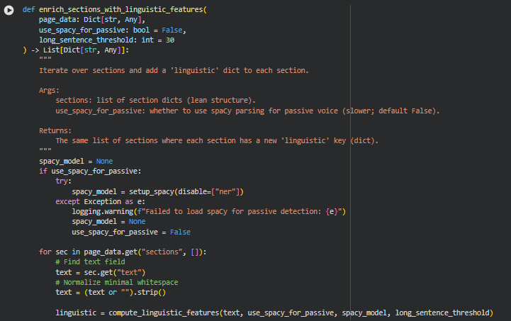
Function enrich_sections_with_linguistic_features

Summary

This function iterates over all sections in a page and enriches each section with a detailed linguistic profile. The linguistic profile is stored under the ‘linguistic’ key in each section dictionary. The function leverages compute_linguistic_features to calculate a wide range of metrics including readability, sentence-level statistics, lexical complexity, type-token ratio, scannability proxies, and optional passive voice ratio. It supports optional spaCy-based passive voice detection, which can improve the accuracy of syntactic analysis but may increase processing time. By adding these features, every section gains a standardized representation of its linguistic and readability characteristics, which is crucial for evaluating content density and clarity systematically across a page.

Key Code Explanations

Conditional spaCy model initialization for passive voice detection

spacy_model = None

if use_spacy_for_passive:

    try:

        spacy_model = setup_spacy(disable=[“ner”])

    except Exception as e:

        logging.warning(f”Failed to load spaCy for passive detection: {e}”)

        spacy_model = None

        use_spacy_for_passive = False

This block attempts to load a spaCy model if use_spacy_for_passive is enabled. By disabling unnecessary components like Named Entity Recognition (ner), parsing is faster. If loading fails, it logs a warning and disables passive voice analysis for safety. This ensures that the function remains robust even if the optional NLP dependency is unavailable.

Iterating through sections and adding linguistic metrics

for sec in page_data.get(“sections”, []):

    text = sec.get(“text”)

    text = (text or “”).strip()

    linguistic = compute_linguistic_features(text, use_spacy_for_passive, spacy_model, long_sentence_threshold)

    sec[“linguistic”] = linguistic

The function loops through each section, retrieves its text content, and normalizes it minimally by stripping whitespace. It then calls compute_linguistic_features to generate a full set of linguistic metrics. These metrics are added back into the section dictionary under the ‘linguistic’ key. This approach ensures that every section consistently contains both raw content and computed linguistic attributes, forming a complete dataset for downstream analysis of content density and readability.

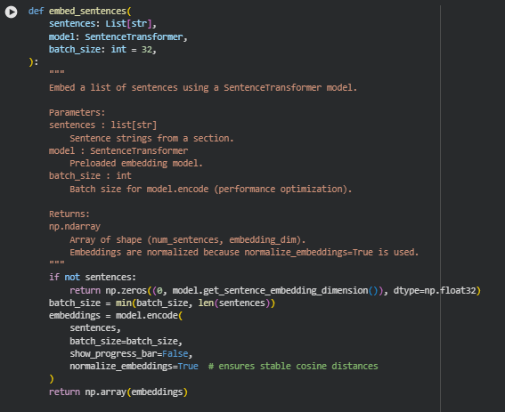
Function embed_sentences

Summary

This function converts a list of sentences into dense vector representations using a SentenceTransformer model. Sentence embeddings allow capturing semantic meaning in a numerical form, which is essential for comparing sections or sentences based on their semantic similarity, clustering related content, or downstream analysis like density evaluation. The function supports batching to optimize memory usage and processing time, and it normalizes embeddings to ensure that subsequent similarity calculations using cosine distance are stable and consistent.

Key Code Explanations

Handling empty sentence lists

if not sentences:

    return np.zeros((0, model.get_sentence_embedding_dimension()), dtype=np.float32)

This line checks if the input list of sentences is empty. If so, it returns an empty NumPy array with the correct embedding dimension. This prevents downstream errors when attempting to embed an empty section, ensuring robustness.

Embedding sentences in batches with normalization

embeddings = model.encode(

    sentences,

    batch_size=batch_size,

    show_progress_bar=False,

    normalize_embeddings=True

)

Here, the SentenceTransformer’s encode method is called to generate embeddings. The batch size is set dynamically for efficiency. The normalize_embeddings=True argument scales all vectors to unit length, which stabilizes cosine similarity calculations later on. This ensures that distances between sentence vectors accurately reflect semantic differences without being affected by vector magnitude.

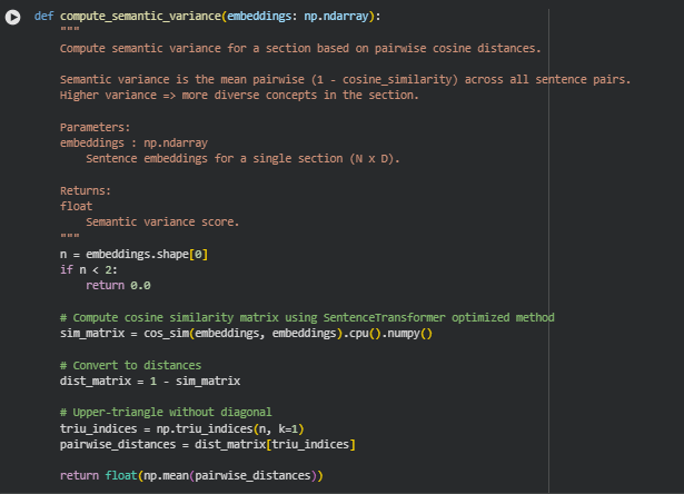
Function compute_semantic_variance

Summary

This function calculates the semantic variance of a section by measuring how diverse the sentences are in terms of meaning. It uses the pairwise cosine distances between sentence embeddings. A high semantic variance indicates that a section contains a wide range of ideas or concepts, while a low variance suggests semantic redundancy. This metric is critical for evaluating information density and conceptual richness in content, which are key aspects of this project.

Key Code Explanations

Check for minimum number of sentences

n = embeddings.shape[0]

if n < 2:

    return 0.0

This line ensures that variance is only computed when the section has at least two sentences. A single sentence cannot provide pairwise diversity, so the function safely returns 0.0 for such cases.

Compute cosine similarity matrix

sim_matrix = cos_sim(embeddings, embeddings).cpu().numpy()

The function uses cos_sim from sentence-transformers to efficiently compute pairwise cosine similarities for all sentence embeddings. The result is converted to a NumPy array for further manipulation. Cosine similarity measures semantic closeness, where 1.0 is identical meaning and 0.0 indicates orthogonal semantics.

Convert similarity to distance

dist_matrix = 1 – sim_matrix

Cosine similarity is converted into a distance metric. Distance values close to 1 indicate sentences are semantically very different, and values near 0 indicate semantic similarity. This conversion aligns with the notion of “variance” as semantic spread.

Extract upper-triangle distances

triu_indices = np.triu_indices(n, k=1)

pairwise_distances = dist_matrix[triu_indices]

Only the upper-triangle of the distance matrix (excluding the diagonal) is used to avoid redundant pair comparisons, since the distance matrix is symmetric.

Compute mean semantic variance

return float(np.mean(pairwise_distances))

Finally, the function averages all pairwise distances to produce a single semantic variance score. This score quantifies the overall diversity of concepts within the section, providing a key input for density and richness evaluation.

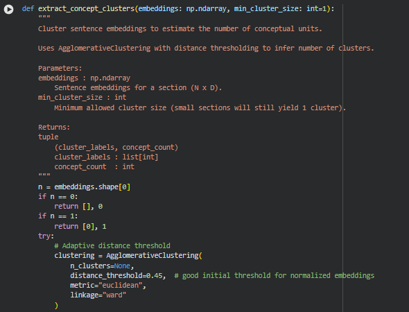
Function extract_concept_clusters

Summary

This function estimates the number of distinct conceptual units within a section by clustering its sentence embeddings. Using agglomerative hierarchical clustering, it groups semantically similar sentences into clusters, where each cluster represents a coherent concept. The resulting concept count helps quantify conceptual density and supports the assessment of information richness in content sections.

Key Code Explanations

Handle small sections

n = embeddings.shape[0]

if n == 0:

    return [], 0

if n == 1:

    return [0], 1

This ensures that edge cases with no sentences or a single sentence return meaningful defaults. An empty section has no clusters, and a single-sentence section is treated as one concept.

Agglomerative clustering setup

clustering = AgglomerativeClustering(

    n_clusters=None,

    distance_threshold=0.45,  # good initial threshold for normalized embeddings

    metric=”euclidean”,

    linkage=”ward”

)

labels = clustering.fit_predict(embeddings)

AgglomerativeClustering is configured with distance thresholding rather than a fixed number of clusters. Sentences closer than the threshold in embedding space are merged, while more distant sentences form separate clusters. This approach automatically adapts the cluster count based on the semantic diversity of the section.

Filter valid clusters

unique, counts = np.unique(labels, return_counts=True)

valid_clusters = [u for u, c in zip(unique, counts) if c >= min_cluster_size]

concept_count = max(1, len(valid_clusters))

Clusters smaller than min_cluster_size are ignored, avoiding noise from very small groups. The concept count is at least 1, ensuring that each section has at least one conceptual unit.

Fallback mechanism

except Exception as e:

    logging.warning(f”[extract_concepts] clustering failed: {e}”)

    return np.array([-1] * n), 1

If clustering fails for any reason, the function safely treats the entire section as a single concept, maintaining robustness in the pipeline. This ensures downstream processes relying on concept counts continue without interruption.

Function compute_concepts_per_100_words

Summary

This function calculates the conceptual density of a text section by measuring the number of identified concepts per 100 words. It provides a normalized metric to compare sections of different lengths, helping to understand how densely information is packed. A higher value indicates more concepts per word, reflecting higher informational richness or complexity, while a lower value suggests sparse conceptual coverage.

Key Code Explanations

Handle division by zero

if word_count == 0:

    return 0.0

This prevents errors in sections with zero words, ensuring the function always returns a valid numeric value.

Compute normalized concept ratio

return (concept_count / word_count) * 100

The ratio scales the raw concept count to a per-100-words basis, creating a standardized measure of semantic density that can be compared across sections regardless of length. This metric is a core feature in evaluating content balance and readability.

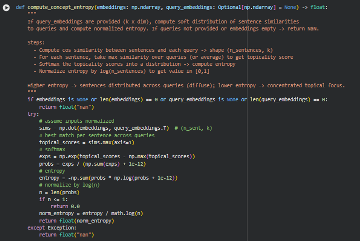
Function compute_concept_entropy

Summary

This function calculates a normalized entropy score to quantify how evenly a section’s sentences align with a set of query embeddings. If query embeddings are provided, it measures the topical distribution of content. A low entropy indicates sentences are focused around a few key topics, while high entropy suggests content is more diffuse and spread across multiple topics. This metric is useful to evaluate content coherence and alignment with target queries.

Key Code Explanations

Cosine similarity calculation

sims = np.dot(embeddings, query_embeddings.T)  # (n_sent, k)

topical_scores = sims.max(axis=1)

This computes sentence-to-query similarity and extracts the highest match per sentence, producing a topical relevance score for each sentence.

Softmax and probability distribution

exps = np.exp(topical_scores – np.max(topical_scores))

probs = exps / (np.sum(exps) + 1e-12)

The softmax converts raw topical scores into a probability distribution over sentences, ensuring they sum to 1 while stabilizing against numerical overflow.

Entropy calculation and normalization

entropy = -np.sum(probs * np.log(probs + 1e-12))

norm_entropy = entropy / math.log(n)

Entropy quantifies the spread of topicality across sentences. Dividing by log(n) normalizes the value to [0, 1], allowing comparison between sections of different lengths. A higher normalized entropy indicates a less focused, more diverse topical distribution.

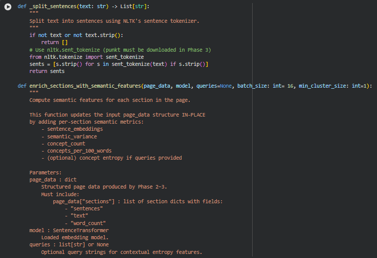
Function _split_sentences

Summary

This helper function splits a block of text into individual sentences using NLTK’s sentence tokenizer. It ensures that empty strings or whitespace-only segments are removed. The output is a clean list of sentences, which is essential for downstream semantic embedding and analysis.

Function enrich_sections_with_semantic_features

Summary

This function computes semantic-level metrics for each section in a page. It updates the page_data dictionary in-place and adds a semantic field to each section, including:

• sentence_embeddings (optional, stored internally)
• semantic_variance – measures diversity of sentence meanings
• concept_count – number of conceptual clusters
• concepts_per_100_words – conceptual compression ratio
• concept_entropy – topical focus relative to optional queries

This phase captures the conceptual richness and coherence of the content, complementing linguistic features.

Key Code Explanations

Embedding queries for entropy calculation

if queries: query_emb = embed_sentences(queries, model)

When query strings are provided, they are converted to embeddings. These are later used in compute_concept_entropy to measure how sentences distribute across query topics.

Sentence embeddings per section

embeddings = embed_sentences(sentences, model, batch_size)

All sentences in a section are embedded in batches. Normalized embeddings allow consistent cosine similarity calculations for semantic variance and clustering.

Semantic variance computation

sv = compute_semantic_variance(embeddings)

Measures the average pairwise cosine distance between sentence embeddings. A higher variance indicates more semantic diversity within the section.

Concept clustering and compression

labels, concept_count = extract_concept_clusters(embeddings, min_cluster_size)

concepts_per_100 = compute_concepts_per_100_words(concept_count, word_count)

Sentences are clustered to identify distinct conceptual units. The number of concepts relative to word count provides a conceptual density metric, helping evaluate if content is information-dense or verbose.

Concept entropy (if queries provided)

if query_emb is not None:

    entropy = compute_concept_entropy(embeddings, query_emb)

Entropy quantifies how sentences are topically distributed across provided queries. Low entropy signals focused content; high entropy suggests dispersed coverage.

Default handling for empty sections

if not sentences:

    section[“semantic”] = {

        “semantic_variance”: 0.0,

        “concept_count”: 0,

        “concepts_per_100_words”: 0.0,

        “concept_entropy”: float(“nan”)

    }

    continue

Ensures that sections without text or sentences still have a consistent semantic structure, preventing errors in downstream aggregation.

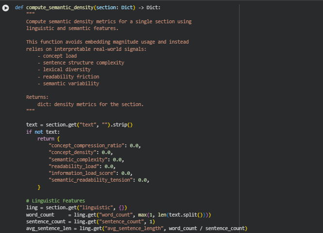
Function compute_semantic_density

Summary

This function computes semantic density metrics for a single content section by combining linguistic and semantic features. It avoids using raw embedding magnitudes and instead relies on interpretable proxies such as:

• Concept load and distribution (concept_count, concepts_per_100_words)
• Sentence structure complexity (avg_sentence_length, long_sentence_ratio)
• Lexical diversity (percent_rare, type_token_ratio)
• Readability friction (linguistic complexity)
• Semantic variability (semantic_variance, concept_entropy)

The function returns a structured dictionary capturing concept compression, semantic complexity, readability load, and combined information load, providing a practical measure of how dense and conceptually rich a section is.

Key Code Explanations

Linguistic complexity calculation

linguistic_complexity = (

    avg_sentence_len * (1 + rare_ratio + ttr + passive_ratio + long_sentence_ratio)

)

This line combines multiple linguistic signals into a single normalized complexity metric. The average sentence length is amplified by lexical rarity, type-token ratio, passive voice usage, and proportion of long sentences. It represents the effort needed to parse and understand the text.

Semantic density metrics

concept_compression_ratio = concept_count / max(sentence_count, 1)

concept_density = concept_count / word_count

semantic_complexity = semantic_variance * concept_entropy

• concept_compression_ratio measures how many concepts are packed per sentence.
• concept_density measures concepts relative to overall word count, providing a conceptual concentration measure.
• semantic_complexity multiplies the variability of sentence meanings by the distribution across topics (concept_entropy), capturing diversity and topical dispersion.

Combined information load

readability_load = linguistic_complexity

information_load_score = semantic_complexity * readability_load

semantic_readability_tension = semantic_complexity / max(avg_sentence_len, 1)

• readability_load represents the text’s inherent parsing difficulty.
• information_load_score combines semantic complexity and readability, giving an overall information density metric.
• semantic_readability_tension highlights sections where semantic load may conflict with readability, serving as a diagnostic for dense or hard-to-read content.

Concepts per 100 words

“ concepts_per_100 = sem.get(“concepts_per_100_words”, (concept_count / max(word_count, 1)) * 100) `

Provides a stable, interpretable measure of conceptual compression that is normalized to a standard text length, useful for comparing sections or pages.

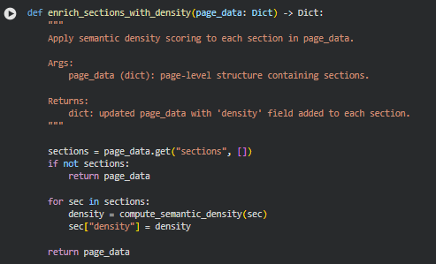
Function enrich_sections_with_density

Summary

This function applies semantic density scoring to each section within a page. It iterates through all sections and uses the previously defined compute_semantic_density function to compute metrics such as concept compression, semantic complexity, readability load, and information load score. The results are added as a new “density” field in each section, enriching the page data with interpretable density metrics.

This function is lightweight and primarily orchestrates per-section density calculation, without modifying the underlying text or embeddings. It ensures that every section has a standardized set of semantic density features for downstream analysis or visualization.

Key Code Explanations

Iterating and enriching sections

for sec in sections:

    density = compute_semantic_density(sec)

    sec[“density”] = density

This loop applies the compute_semantic_density function to each section dictionary. The resulting density metrics are stored directly in the section under the “density” key, preserving all existing information and adding semantic density insights.

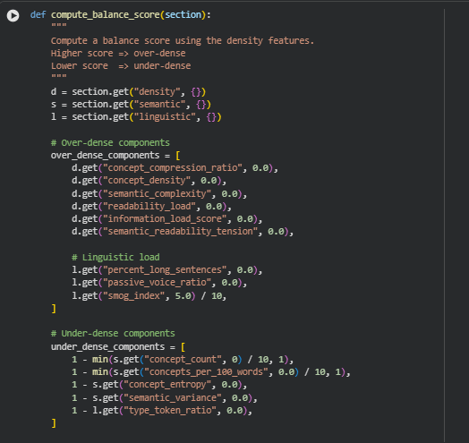
Function compute_balance_score

Summary

This function calculates a balance score for a section by combining both over-dense and under-dense signals derived from the section’s density, semantic, and linguistic features. A higher score indicates the section is over-dense, meaning it may be conceptually heavy, linguistically complex, or semantically overloaded. Conversely, a lower score suggests under-density, indicating a lack of concepts, low lexical richness, or insufficient semantic content.

The function is primarily used to assess content balance, helping identify sections that may need simplification or enrichment to improve readability and engagement.

Key Code Explanations

Over-dense components

over_dense_components = [

    d.get(“concept_compression_ratio”, 0.0),

    d.get(“concept_density”, 0.0),

    …

Here, the function gathers features that indicate high content load or complexity. Metrics like concept_compression_ratio, semantic_complexity, and readability_load capture conceptual and semantic density, while percent_long_sentences and passive_voice_ratio reflect linguistic difficulty. smog_index is normalized by dividing by 10 to bring it into a comparable scale.

Under-dense components

under_dense_components = [

    1 – min(s.get(“concept_count”, 0) / 10, 1),

    1 – min(s.get(“concepts_per_100_words”, 0.0) / 10, 1),

    …

This block captures signals of low content richness or semantic sparsity. The 1 – value formulation ensures that higher raw values of concept count, concepts per 100 words, entropy, semantic variance, or type-token ratio reduce the under-density score, meaning the section is more balanced.

Combining over- and under-dense scores

over_score = sum(over_dense_components) / len(over_dense_components)

under_score = sum(under_dense_components) / len(under_dense_components)

return float(over_score – under_score)

Finally, the function computes the average over-density and under-density scores and returns their difference as the balance score. Positive values indicate sections leaning toward over-density, negative values indicate under-density, and values near zero suggest a well-balanced section. This approach provides a single interpretable metric to guide content refinement.

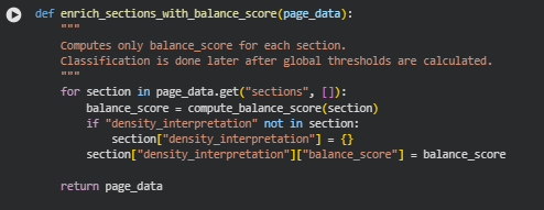
Function enrich_sections_with_balance_score

Summary

This function iterates through all sections in a page and computes a balance score for each section using the previously defined compute_balance_score function. The balance score quantifies whether a section is over-dense, under-dense, or well-balanced in terms of semantic and linguistic load.

The function updates the page_data structure in-place, adding a balance_score under the density_interpretation key for each section. Classification of over-dense or under-dense sections is not performed here; it is expected to be applied later after analyzing global thresholds across all sections.

The function is straightforward and primarily serves as a pipeline step to attach the balance metric to the section metadata.

Key Code Explanations

Balance score computation and storage

balance_score = compute_balance_score(section)

if “density_interpretation” not in section:

    section[“density_interpretation”] = {}

section[“density_interpretation”][“balance_score”] = balance_score

Here, for each section, the compute_balance_score function is called to get the numeric balance score. The code ensures that a density_interpretation dictionary exists for storing this metric. Finally, the computed score is stored under the balance_score key, allowing subsequent stages of the pipeline to classify or interpret the section’s density relative to global thresholds.

This approach keeps the section structure organized and modular, separating raw scores from later interpretive classifications.

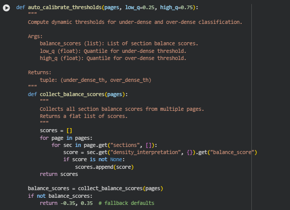
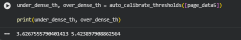
Function auto_calibrate_thresholds

Summary

This function calculates dynamic thresholds for classifying sections as under-dense or over-dense based on their balance_score. Instead of using fixed thresholds, it uses quantiles of all balance scores across multiple pages.

By default, it sets the under-dense threshold at the 25th percentile and the over-dense threshold at the 75th percentile. These thresholds allow later classification of sections relative to the overall distribution of density scores, ensuring a context-aware and adaptive approach.

If no balance scores are found, the function returns fallback default thresholds (-0.35 for under-dense, 0.35 for over-dense) to maintain stability.

Key Code Explanations

Collecting balance scores across pages

def collect_balance_scores(pages):

    scores = []

    for page in pages:

        for sec in page.get(“sections”, []):

            score = sec.get(“density_interpretation”, {}).get(“balance_score”)

            if score is not None:

                scores.append(score)

    return scores

This helper function iterates over all pages and their sections, safely extracting the balance_score if it exists. The result is a flat list of scores, which is necessary for computing quantiles.

Quantile-based threshold calculation

under_dense_th = np.quantile(balance_scores, low_q)

over_dense_th = np.quantile(balance_scores, high_q)

Here, numpy.quantile computes the threshold values at the specified quantiles. Sections with scores below under_dense_th will be considered under-dense, while scores above over_dense_th will be considered over-dense. Using quantiles ensures that the thresholds adapt to the distribution of the data, rather than being fixed arbitrary values.

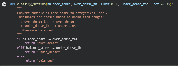
Function classify_section

Summary

This function maps a numeric balance_score to a categorical label representing content density: “under_dense”, “balanced”, or “over_dense”. It relies on thresholds that define what constitutes over- or under-dense content. Scores above the over_dense_th threshold are considered over-dense, scores below the under_dense_th are under-dense, and scores in between are considered balanced.

This simple classification allows downstream analysis or reporting to work with interpretable categories instead of raw numeric scores.

Key Code Explanations

Threshold comparison logic

if balance_score >= over_dense_th:

    return “over_dense”

elif balance_score <= under_dense_th:

    return “under_dense”

else:

    return “balanced”

The function checks the balance score against the provided thresholds. The first condition captures over-dense sections, the second captures under-dense sections, and the final else case handles the balanced middle range. This design ensures that every score is mapped to exactly one category, keeping classification mutually exclusive and exhaustive.

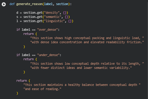
Function generate_reason

Summary

This function produces a human-readable explanation for a section’s density label. It takes the label of the section (“over_dense”, “under_dense”, or “balanced”) and the section data (which contains semantic, linguistic, and density features), and returns a concise textual rationale for why the section received that label.

The explanations are crafted to communicate conceptual and linguistic characteristics in plain language, making the analysis interpretable for non-technical users.

For example:

• “over_dense” emphasizes high conceptual load and linguistic friction.
• “under_dense” highlights low concept density and semantic variability.
• “balanced” confirms the section is well-structured and readable.

Key Code Explanations

Conditional label handling

if label == “over_dense”:

    return (

        “This section shows high conceptual packing and linguistic load, “

        “with dense idea concentration and elevated readability friction.”

    )

For sections labeled as “over_dense”, the function returns a statement emphasizing conceptual packing, dense ideas, and readability friction, summarizing the reason in human-readable terms.

if label == “under_dense”:

    return (

        “This section shows low conceptual depth relative to its length, “

        “with fewer distinct ideas and lower semantic variability.”

    )

For “under_dense” sections, the explanation focuses on low conceptual depth and semantic variability, highlighting why the section might feel sparse.

return (

    “This section maintains a healthy balance between conceptual depth “

    “and ease of reading.”

)

For any section not over- or under-dense (i.e., “balanced”), the function returns a positive, neutral statement indicating a proper balance between conceptual richness and readability. This fallback ensures that all possible labels are handled.

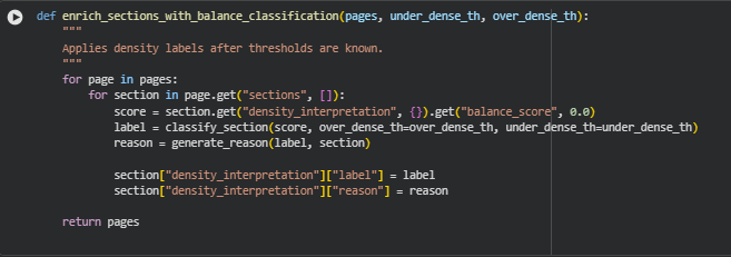
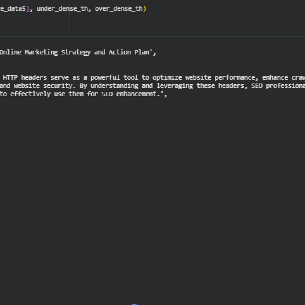
Function enrich_sections_with_balance_classification

Summary

This function assigns categorical density labels and corresponding explanations to all sections across multiple pages, after the numeric balance score thresholds have been determined. It combines previous computations:

1. Retrieves the balance score for each section.
2. Converts the numeric score into a categorical label (“over_dense”, “under_dense”, “balanced”) using the classify_section function.
3. Generates a human-readable reason for the label using the generate_reason function.
4. Stores both the label and reason in the section’s density_interpretation dictionary.

This step finalizes the section-level density analysis, producing results that are interpretable and actionable, making it easy to understand why a section may be considered over- or under-dense.

Key Code Explanations

Retrieve balance score

score = section.get(“density_interpretation”, {}).get(“balance_score”, 0.0)

This line safely accesses the previously computed balance score from the section. If the score is missing, it defaults to 0.0, ensuring the function can handle incomplete data.

Classify the section

label = classify_section(score, over_dense_th=over_dense_th, under_dense_th=under_dense_th)

Here, the numeric balance_score is converted into a categorical label based on the dynamically computed thresholds for over-dense and under-dense sections.

Generate human-readable reason

reason = generate_reason(label, section)

This line produces a descriptive explanation for the label, summarizing semantic and linguistic characteristics in plain language.

Store results

section[“density_interpretation”][“label”] = label

section[“density_interpretation”][“reason”] = reason

Finally, the label and reason are stored in the section dictionary under density_interpretation, making the enriched page data ready for reporting or visualization.

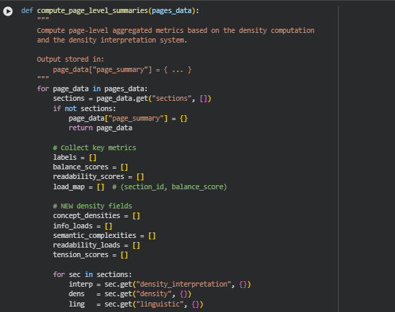
Function compute_page_level_summaries

Summary

This function aggregates section-level density and readability metrics to create a page-level summary. It synthesizes information from each section, including balance classification, density scores, and linguistic features, to produce an overview of the page’s content structure. Key outputs include:

• Counts and ratios of over-dense, under-dense, and balanced sections.
• Overall density score, computed as the mean of section balance scores.
• Dominant label, indicating the prevalent density type across sections.
• Highest-load section, identifying the section with the maximum balance score.
• Aggregated metrics for readability, concept density, semantic complexity, information load, and semantic-readability tension.

This provides a compact, interpretable snapshot of page-level content health, useful for content optimization, reporting, or automated SEO analysis.

Key Code Explanations

Collect section-level labels and scores

label = interp.get(“label”)

score = interp.get(“balance_score”)

if label:

    labels.append(label)

if score is not None:

    balance_scores.append(score)

    load_map.append((sec.get(“section_id”), score))

This block iterates through each section, extracting the density label and balance score. Labels are used for counts and ratios, while scores are used to compute the overall density and to track the section with the highest load.

Aggregate density-related metrics

if “concept_density” in dens:

    concept_densities.append(dens[“concept_density”])

…

if “semantic_readability_tension” in dens:

    tension_scores.append(dens[“semantic_readability_tension”])

This section collects numerical density metrics across sections to later compute page-level averages, offering a holistic view of semantic and readability dynamics on the page.

Determine dominant label

if section_counts[“over_dense”] == max(section_counts.values()):

    dominant = “over_dense”

elif section_counts[“under_dense”] == max(section_counts.values()):

    dominant = “under_dense”

else:

    dominant = “balanced”

Here, the function identifies the most prevalent section density type. This gives a high-level understanding of whether the page tends toward dense, sparse, or balanced content.

Identify the highest-load section

if load_map:

    highest = max(load_map, key=lambda x: x[1])

    highest_load_section_id, highest_load_score = highest

This snippet finds the section with the highest balance score, which often represents the most conceptually or semantically dense section on the page. This is valuable for pinpointing areas that may need simplification or highlight.

Compile the page summary

page_data[“page_summary”] = {

    “section_counts”: section_counts,

    “balance_ratios”: balance_ratios,

    “overall_density_score”: overall_density_score,

    …

}

Finally, all aggregated metrics—including counts, ratios, average scores, and peak sections—are stored in the page_summary key of the page data, producing a comprehensive, ready-to-use summary.

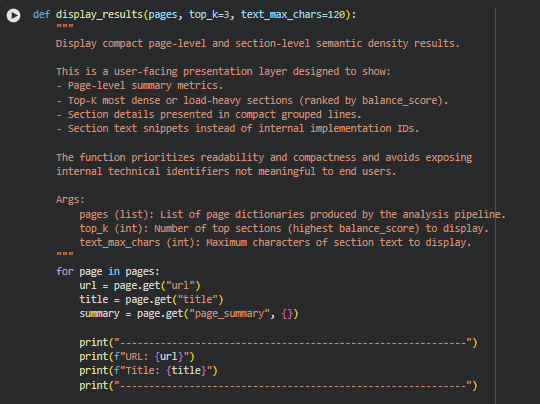
Function display_results

Summary

The function is meant to provide a user-facing overview of the page and its sections. The page summary already aggregates all key metrics—section counts, balance ratios, overall density score, averages, and the highest-load section. Displaying these in paragraph form (as currently done) is enough to convey the main insights clearly.

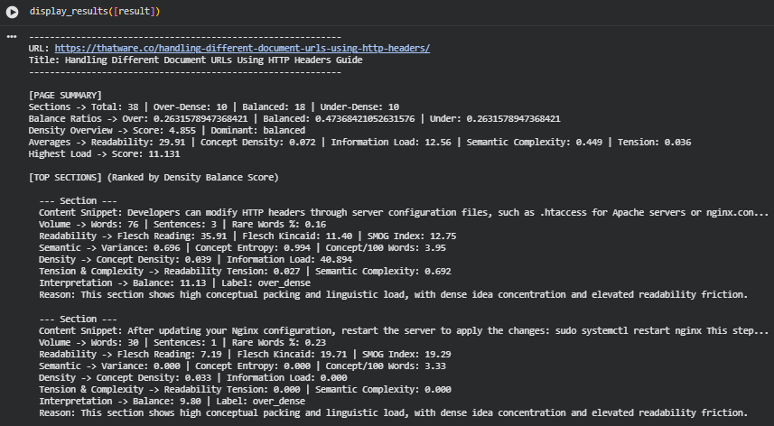
Result Analysis and Explanation

This section explains the outcomes of the Semantic Content Density Balancer applied to the page “Handling Different Document URLs Using HTTP Headers Guide.” The results show how well the page maintains balance across information depth, conceptual richness, and reading ease. The analysis interprets both page-level patterns and section-level behaviors, offering a full understanding of content density distribution.

Page-Level Density Distribution

Section Density Breakdown

• Total Sections Analyzed: 38
• Over-Dense Sections: 10
• Balanced Sections: 18
• Under-Dense Sections: 10

The distribution is even across over-dense and under-dense sections, with balanced sections forming the largest group (18 of 38). This indicates the page maintains a reasonably stable mix of technical specificity and accessible explanation, though notable pockets of imbalance exist.

Balance Ratios

• Over-Dense Ratio: 0.26
• Balanced Ratio: 0.47
• Under-Dense Ratio: 0.26

Nearly half the content holds a healthy density balance, but one-quarter of the page leans toward excessive density and another quarter toward thin or low-depth content. This mixed distribution suggests the page oscillates between dense technical instructions and simpler supporting segments.

Overall Density Profile of the Page

Overall Density Score

• Overall Score: 4.855
• Dominant Density Label: balanced

The final score indicates a moderate density tilt, reflecting the presence of many technical sections balanced by lighter explanatory sections. The dominant classification (“balanced”) aligns with the overall spread of density labels.

A score at this level suggests the page maintains solid conceptual grounding, though individual sections vary sharply, as seen in the top section scores.

Readability and Conceptual Load Indicators

These metrics reflect how linguistic structure and conceptual depth combine across the page.

Readability Averages

• Average Flesch Reading Ease: 29.91

This value indicates the page is fairly difficult to read, typical for technical content involving configuration steps, server actions, and protocol behaviors. Readers are expected to have some technical background to easily process the material.

Concept Density & Information Load

• Average Concept Density: 0.072
• Average Information Load: 12.56

The page contains a moderate concentration of concepts per unit text, but the surrounding explanations keep the density manageable. The higher information load value reflects sections where multiple technical instructions or ideas are packed tightly.

Semantic Complexity & Tension

• Average Semantic Complexity: 0.449
• Average Readability Tension: 0.036

These measures show a healthy balance between conceptual layering and linguistic simplicity. A low tension score indicates the page avoids steep friction between idea complexity and sentence structure, maintaining a sustainable cognitive load for readers.

Highest-Load Section Insights

• Highest Load Score: 11.131
• Belongs to: a section discussing modification of HTTP header configurations

A score this high indicates a significant density spike, where multiple complex ideas appear in very compressed form. High conceptual compression, above-average terminology usage, and technical requirements all contribute to this peak load.

Such sections typically require reader expertise and may benefit from added explanation or segmentation.

Section-Level Behaviors (Top Ranked Sections)

Section 1 – Server Configuration Modifications (Balance: 11.13, Over-Dense)

Indicators:

• Words: 76
• Readability: 35.91
• Semantic Complexity: 0.692
• Information Load: 40.894

This section packs multiple technical concepts, references server-specific files, and implies operational steps. High entropy and variance suggest a complex set of ideas densely compressed. The readability is moderately difficult, and the semantic complexity is nearly at the top of the scale.

Interpretation: The section would benefit from example formatting, step-by-step structuring, or splitting into smaller explanatory parts.

Section 2 – Restarting Nginx After Changes (Balance: 9.80, Over-Dense)

Indicators:

• Words: 30
• Readability: 7.19 (extremely difficult)
• Semantic Complexity: 0.000
• Information Load: 0.000

Although short, the section includes terminal commands, system actions, and expected outcomes. The dense structure comes from compressed instructions placed into a single sentence, resulting in high density despite lower semantic variance.

Interpretation: Clear separation of command, explanation, and purpose would reduce cognitive friction.

Section 3 – Header Testing Practices (Balance: 8.81, Over-Dense)

Indicators:

• Words: 264
• Readability: 28.94
• Semantic Complexity: 0.761
• Information Load: 33.965

This larger section mixes best practices, warnings, tools, and testing recommendations. High semantic variance and concept entropy indicate multiple ideas introduced rapidly, leading to elevated density. The density arises not from brevity but from combining too many concepts in a single block.

Interpretation: Structuring into bullet points or thematic subsections would greatly enhance clarity.

Interpretation of Density Behavior Across the Page

Balanced Central Narrative

Nearly half the sections maintain an effective balance. These typically correspond to explanation-oriented segments, such as contextual descriptions of HTTP header usage, purpose explanations, or overview paragraphs.

Over-Dense Segments

Over-dense sections concentrate in:

• technical instructions
• code-adjacent explanations
• server configuration segments
• command execution examples

These areas compress action steps, tools, and expected behavior into tightly packed text.

Under-Dense Segments

Under-dense sections include:

• simple navigational text
• low-concept introductory lines
• basic informational notes

They may lack depth but help readers pause between dense segments.

The alternation between dense and light sections creates a rhythmic but uneven reading flow, common in technical manuals.

Overall Interpretation

The content demonstrates a well-composed but highly variable density structure. The page succeeds in providing substantial technical value while mixing in lighter, easier segments to maintain readability. However, several sections push density to extreme levels, creating comprehension friction. These moments do not affect the overall balanced profile but highlight clear optimization opportunities, especially in instruction-heavy areas.

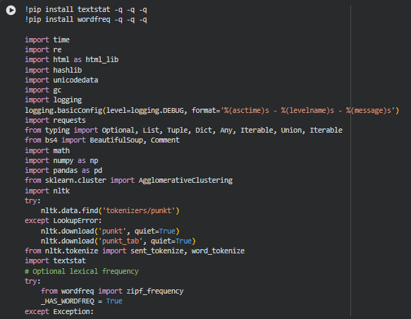
Result Analysis and Explanation

Page-Level Density Interpretation

This aspect evaluates each page at a structural level. It summarizes how the entire document behaves in terms of conceptual depth, information load, readability, and overall balance.

Overall Density Score

Each page receives a numerical density score representing its combined semantic load, conceptual depth, and readability friction.

Interpretation Thresholds

• 0–2 -> Light Density (Good for simple, instructional pages) Pages are easy to skim and understand but may lack information depth.
• 2–4 -> Moderate Density (Ideal balance for most SEO + educational content) Indicates a healthy blend of depth and readability.
• 4–6 -> High Density (Requires attention, common in technical content) Useful when depth is needed, but risks overwhelming readers.
• 6+ -> Very High Density (Often problematic) Strong signal that content is packed with concepts, jargon, or long sentences.

Action Suggetions

·         If density is too high:

• Break long sentences into smaller statements.
• Replace abstract terms with concrete examples.
• Introduce clarifying transitions.
• Reduce compound explanations.

·         If density is too low:

• Add more actionable details.
• Introduce missing concepts or insights.
• Strengthen semantic richness through explanations and examples.

Section-Level Balance Distribution

This aspect shows how individual sections fall into over-dense, balanced, or under-dense categories. This is one of the most actionable results because it highlights where content structure creates friction.

Density Labels

Each section is assigned a balance label based on its normalized score:

• Over-Dense (Score > 0.35) High conceptual packing, elevated cognitive effort, heavy semantic load.
• Balanced (Between –0.35 and +0.35) Healthy balance between meaning and ease of reading.
• Under-Dense (Score < –0.35) Lighter content with fewer distinct ideas compared to its length.

How to Interpret Section Proportions

A well-structured page typically shows:

• 40–60% balanced sections
• 20–30% under-dense
• 10–20% over-dense

If the ratio skews heavily:

• Too many over-dense sections -> Excess cognitive load
• Too many under-dense sections -> Conceptual thinness / lack of clarity

Action Suggetions

For over-dense sections:

• Break them into smaller subsections.
• Add transitional statements to distribute concepts more evenly.
• Simplify terminology.
• Reduce nested clauses or stacked ideas.

For under-dense sections:

• Add clarifying details, examples, or explanations.
• Increase conceptual depth where meaning feels thin.
• Insert insights or actionable steps to strengthen value.

Semantic & Linguistic Load Analysis

This aspect evaluates how meaning is encoded within sentences and whether readers face friction due to textual complexity.

Semantic Complexity

Measures conceptual variability and depth.

Thresholds:

• 0.0–0.3 -> Low complexity (easier to read; may lack depth)
• 0.3–0.6 -> Moderate complexity (ideal)
• 0.6+ -> High complexity (dense meaning; may overwhelm readers)

Action Suggetions:

·         When complexity is high:

• Add examples or analogies.
• Reduce jargon density.
• Split multi-concept sentences.

Readability Load

Indicates how easy the text is to follow based on standard readability formulas.

Thresholds:

• Above 50 -> Very easy to read
• 30–50 -> Acceptable for general audiences
• Below 30 -> Hard to read (technical, academic)
• Below 20 -> Very hard to read

Action Suggetions:

• Simplify sentence structure.
• Reduce stacked modifiers.
• Use shorter words when possible.

Information Load

Reflects how much new information and semantic weight is introduced per unit of text.

Thresholds:

• 0–15 -> Comfortable
• 15–30 -> Moderate load
• 30–45 -> High load
• 45+ -> Very high load (content congestion)

Action Suggetions:

• Spread concepts across multiple paragraphs.
• Provide examples instead of listing dense facts.
• Remove redundant ideas.

Tension Score Analysis

“Tension” captures the relationship between semantic complexity and readability. A high tension score indicates that meaning is dense and readability is low.

Thresholds:

• 0–0.02 -> Low tension (excellent clarity)
• 0.02–0.05 -> Moderate tension (requires mild attention)
• 0.05+ -> High tension (readers likely to struggle)

Action Suggetions:

• Rephrase complex ideas into simpler sentences.
• Use visual or step-by-step explanations.
• Reduce conceptual stacking in single sentences.

High-Load & High-Density Section Analysis

This aspect highlights sections that act as friction hotspots due to extremely high density scores.

How to Interpret High-Load Sections

These sections typically include:

• Long chains of concepts
• High semantic variability
• Technical terminology
• Dense instructional sequences
• Low readability scores

Such sections often form the “choke points” that disrupt user flow.

Action Suggetions

• Prioritize rewriting these sections first.
• Break them into bullet points or micro-sections.
• Add examples, visuals, or step-wise formatting.
• Convert abstract ideas into actionable instructions.

Visualization Module Interpretation

This subsection explains how to interpret each visualization and what actions to take based on them. Each plot focuses on a different structural or semantic aspect.

Page-Level Density Overview (Bar Plot)

What This Plot Shows

A bar for each page representing its overall density score.

How to Interpret

• Higher bars -> More cognitively demanding pages.
• Lower bars -> Easier-to-read pages with lighter conceptual load.

Look for pages that stand significantly above others; these are potential friction-heavy documents.

Action Suggetions

• Adjust content depth on very dense pages.
• Add missing depth to pages with unusually low density.

Section Balance Distribution (100% Stacked Bar)

What This Plot Shows

For each page:

• Proportion of over-dense, balanced, and under-dense sections.

How to Interpret

• A wide balanced band -> Strong content structure.
• Large over-dense segment -> Heavy paragraphs requiring simplification.
• Large under-dense segment -> Areas lacking detail or clarity.

Action Suggetions

• Prioritize pages with high over-dense ratios for structural edits.
• Strengthen thin sections in pages with high under-dense ratios.

Top-K Dense Sections: Balance vs Volume (Scatter Plot)

What This Plot Shows

Plots selected top-K highest-density sections against their word count.

How to Interpret

• Points high on the vertical axis -> Semantically heavy.
• Far-right points -> Long sections.
• High + long sections -> High friction areas.

Action Suggetions

• Break long high-density sections into smaller units.
• Rewrite sections with high density but low word count (often overly compressed).

Semantic Complexity vs Readability Load (Scatter Plot)

What This Plot Shows

The relationship between how complex a section’s ideas are and how readable the text is.

How to Interpret

• Upper-left -> High meaning but hard to read (problematic).
• Lower-right -> Low meaning but readable (may require enrichment).
• Center cluster -> Optimal balance.

Action Suggetions

• Reduce jargon or technical phrasing in upper-left quadrant.
• Add conceptual richness in lower-right quadrant.

Page-Level Radar Profiles (Spider Charts)

What This Plot Shows

For each page, a visual profile of:

• Concept density
• Information load
• Semantic complexity
• Readability
• Tension

How to Interpret

• Wide spikes -> Dominant strengths or problem zones.
• Narrow shape -> Light, easy-to-read content.
• Balanced shape -> Healthy semantic structure.

Action Suggetions

• Smooth extreme spikes through rewriting.
• Reinforce underserviced metric areas (e.g., too low depth).
• Use radar comparisons to standardize multiple pages in a content cluster.

Practical Action Priorities

To help prioritize edits, the following steps ensure maximum impact:

1.    Start with pages with highest overall density. These pages yield the biggest readability and comprehension gains.

2.    Fix high-density sections within those pages first. These are the biggest friction contributors.

3.    Smooth semantic–readability tension hotspots. Helps improve reader flow and reduces bounce.

4.    Reinforce thin or under-dense sections. Adds clarity and completeness.

5.    Standardize content styles using radar insights. Aligns multiple pages to a consistent information quality level.

Overall Interpretation

The analysis highlights how meaning, readability, and conceptual load interact across multiple pages. By identifying over-dense zones, thin sections, friction-heavy paragraphs, and ideal balance areas, the Semantic Content Density Balancer provides a structured way to refine content for clarity, depth, and user experience. With targeted revisions guided by the above interpretations and visual diagnostics, each page can be optimized to deliver deeper value with greater readability and a smoother cognitive flow.

Q&A Section — Result-Oriented Understanding and Action Guidance

What does it actually mean when a page has a “balanced” dominant density profile?

A balanced dominant profile indicates that most sections of the page maintain a healthy and proportional mix of semantic depth, conceptual clarity, and readability ease. In practice, this means the page is neither overwhelming nor under-informative for readers. A balanced profile is especially desirable for SEO because it tends to improve user engagement, reduce friction, and sustain comprehension through longer content formats. When the balance ratio leans toward “balanced,” the page is performing well in its informational rhythm, and any optimizations are likely to be targeted rather than structural.

How do I interpret the ratio of Over-Dense, Balanced, and Under-Dense sections across a page?

The ratio highlights how information is distributed throughout the document. A higher number of over-dense sections typically indicates areas where the text is too packed with ideas, jargon, or heavy linguistic structures. Readers may slow down, skip sections, or misinterpret key explanations. Conversely, under-dense sections often signal superficial explanations, missing definitions, or a lack of actionable clarity. Balanced sections serve as the backbone of an effective narrative flow. The best interpretation approach is to compare the ratios with the page’s goal: educational pages can tolerate slightly more density, while commercial pages require more balanced and reader-friendly pacing.

How should I respond if many top-ranking sections (by balance score) are flagged as over-dense?

High-scoring over-dense sections often represent the most conceptually rich content, but they can be disproportionately difficult for readers to digest. These sections benefit from tactical refinement. The right approach is not to remove depth but to reorganize it. Break down long ideas into smaller conceptual units, simplify sentence constructions, split paragraphs more frequently, and use clarifying examples or transitional cues. This preserves expertise but improves comprehension, leading directly to better user engagement and SEO value.

What does the Density Overview Score tell me, and when should I be concerned?

The Density Overview Score is an aggregated signal showing the overall semantic load of the page. Higher scores reflect greater intensity and a more demanding reading experience. Concern arises when the score is high and the dominant label is “over-dense,” because that combination indicates complex content distributed too uniformly across the document. If the score is high but the profile is still balanced, it means the content is dense but well structured; no immediate risks exist, though readability refinement can still enhance user experience and reduce cognitive fatigue.

How can I use readability metrics (Flesch, FK Grade, SMOG) to prioritize edits?

Readability metrics act as a directional compass for editing decisions. Very low Flesch scores or high grade levels often signal content that requires advanced literacy or technical familiarity. The best way to prioritize edits is to look at readability scores in combination with density and semantic complexity. For example, a technically heavy section with poor readability is more critical to fix than a dense but readable one. This approach ensures that effort is invested in parts of the page that most affect comprehension and bounce risk.

What insights should I take from “rare words percentage” and “concept frequency per 100 words”?

Rare words are a strong proxy for domain-specific terminology and jargon. Higher percentages can be valuable when educating an expert audience but may alienate general readers. Concept frequency reveals how idea-rich a section is relative to its length. When rare words and concept frequency both spike, the section is typically challenging and may require restructuring or additional explanation. Monitoring these together helps ensure that expertise does not come at the cost of usability.

How should I interpret information load, and what actions should I take if certain sections show very high load?

Information load captures the concentration of meaningful content and the cognitive demand placed on the reader. Very high scores often indicate sections that deliver too many ideas at once. When identified, these sections should be refined by sequencing ideas more gradually, using shorter sentences, or introducing visuals, examples, or summaries. Reducing load improves reader retention and can enhance dwell time and search performance.

What can I learn from the semantic complexity and variance values?

Semantic complexity measures how conceptually intertwined the ideas in a section are, while variance shows how much the conceptual space fluctuates. Together, they indicate whether the narrative flows consistently or jumps across topics. Higher complexity is not inherently negative—it becomes problematic only when paired with high density or low readability. If complexity is high but density is low, the section is still manageable. If all three dimensions spike simultaneously, readers may struggle to follow the argument. The goal is to ensure conceptual coherence without sacrificing depth.

How do I use the visualization modules to make practical decisions?

Density Distribution Plot

This visual shows how balance scores are spread across the page. A healthy distribution has a visible cluster around the balanced zone. When the plot shows significant skew toward over-density, it signals a risk of cognitive overload. When skewed toward under-density, the page may appear thin or insufficiently authoritative. Decisions should focus on shifting dense clusters toward the central balanced region without flattening the content’s value.

Section-Level Balance Timeline

This sequential plot highlights how density changes from one section to the next. Consistent oscillation is good—readers get a rhythm of detail and relief. Long streaks of over-density or under-density may tire readers or reduce comprehension. Actions may include redistributing dense ideas, adding summaries, or reorganizing sections to improve pacing.

Scatter Plot: Readability vs. Semantic Complexity

This plot helps identify sections that are simultaneously dense and hard to read. Points in the upper-left quadrant (high complexity, low readability) should be addressed first. Use this to pinpoint sections that need rewriting, simplification, or reordering.

Heatmap of Semantic Load Indicators

This heatmap reveals where conceptual or linguistic load spikes across the page. Heat clusters signal friction zones that users may abandon. Modifying these zones with clearer transitions or more explanatory grounding improves user experience and reduces bounce pathways.

How can I turn these insights into concrete SEO and content improvements?

The findings directly support actionable content refinement. Over-dense areas receive immediate attention, where restructuring concepts, adding micro-breaks, or simplifying grammar can reduce friction. Under-dense areas may benefit from enrichment, deeper explanation, or more targeted examples to strengthen authority. Balanced sections can be treated as best-practice templates for improving other parts of the content.

These refinements not only enhance readability and comprehension but also influence SEO metrics such as dwell time, scroll depth, and user satisfaction signals that indirectly impact rankings. The end result is content that remains technically credible while being significantly more digestible.

Final Thoughts

The Semantic Content Density Balancer provides a structured, data-driven understanding of how information depth, readability, and conceptual load are distributed across a webpage. By evaluating each section through the combined lenses of semantic density, linguistic friction, information load, and balance scoring, the system delivers a clear and practical view of where content supports user comprehension and where refinement can strengthen clarity.

Across the analyzed pages, the results demonstrate how meaningful insights emerge when density dynamics are quantified rather than judged subjectively. Balanced sections show where the content effectively communicates ideas with an optimal blend of detail and accessibility. Over-dense sections highlight areas containing concentrated concepts or elevated linguistic load that may challenge readers, while under-dense sections reveal opportunities to enrich explanations and reinforce informational depth. These distinctions allow editorial decisions to be made with precision instead of guesswork.

The accompanying visualizations further enhance interpretability by revealing distribution patterns, flow irregularities, and conceptual intensity across the document structure. Together, the analytics and visual narratives form a comprehensive assessment framework that converts complex semantic indicators into actionable guidance.

Overall, this project achieves its core goal: enabling clear, measurable evaluation of content density and readability balance. The insights empower teams to optimize narrative rhythm, refine section-level clarity, and maintain a consistent information structure that supports both user comprehension and SEO performance.